注意
转到末尾下载完整的示例代码。或者通过 JupyterLite 或 Binder 在浏览器中运行此示例
分位数回归#
本示例说明了分位数回归如何预测非平凡的条件分位数。
左图显示了误差分布为正态但方差不恒定的情况,即存在异方差性。
右图显示了一个非对称误差分布的示例,即帕累托分布。
# Authors: The scikit-learn developers
# SPDX-License-Identifier: BSD-3-Clause
数据集生成#
为了说明分位数回归的行为,我们将生成两个合成数据集。这两个数据集的真实生成随机过程都将由相同的期望值组成,并与单个特征 x 呈线性关系。
import numpy as np

rng = np.random.RandomState(42)
x = np.linspace(start=0, stop=10, num=100)
X = x[:, np.newaxis]
y_true_mean = 10 + 0.5 * x
我们将通过改变目标 y 的分布来创建两个后续问题,同时保持相同的期望值
第一种情况是添加异方差正态噪声;
第二种情况是添加非对称帕累托噪声。
y_normal = y_true_mean + rng.normal(loc=0, scale=0.5 + 0.5 * x, size=x.shape[0])
a = 5
y_pareto = y_true_mean + 10 * (rng.pareto(a, size=x.shape[0]) - 1 / (a - 1))
我们首先可视化数据集以及残差 y - mean(y) 的分布。
import matplotlib.pyplot as plt

_, axs = plt.subplots(nrows=2, ncols=2, figsize=(15, 11), sharex="row", sharey="row")

axs[0, 0].plot(x, y_true_mean, label="True mean")
axs[0, 0].scatter(x, y_normal, color="black", alpha=0.5, label="Observations")
axs[1, 0].hist(y_true_mean - y_normal, edgecolor="black")


axs[0, 1].plot(x, y_true_mean, label="True mean")
axs[0, 1].scatter(x, y_pareto, color="black", alpha=0.5, label="Observations")
axs[1, 1].hist(y_true_mean - y_pareto, edgecolor="black")

axs[0, 0].set_title("Dataset with heteroscedastic Normal distributed targets")
axs[0, 1].set_title("Dataset with asymmetric Pareto distributed target")
axs[1, 0].set_title(
    "Residuals distribution for heteroscedastic Normal distributed targets"
)
axs[1, 1].set_title("Residuals distribution for asymmetric Pareto distributed target")
axs[0, 0].legend()
axs[0, 1].legend()
axs[0, 0].set_ylabel("y")
axs[1, 0].set_ylabel("Counts")
axs[0, 1].set_xlabel("x")
axs[0, 0].set_xlabel("x")
axs[1, 0].set_xlabel("Residuals")
_ = axs[1, 1].set_xlabel("Residuals")
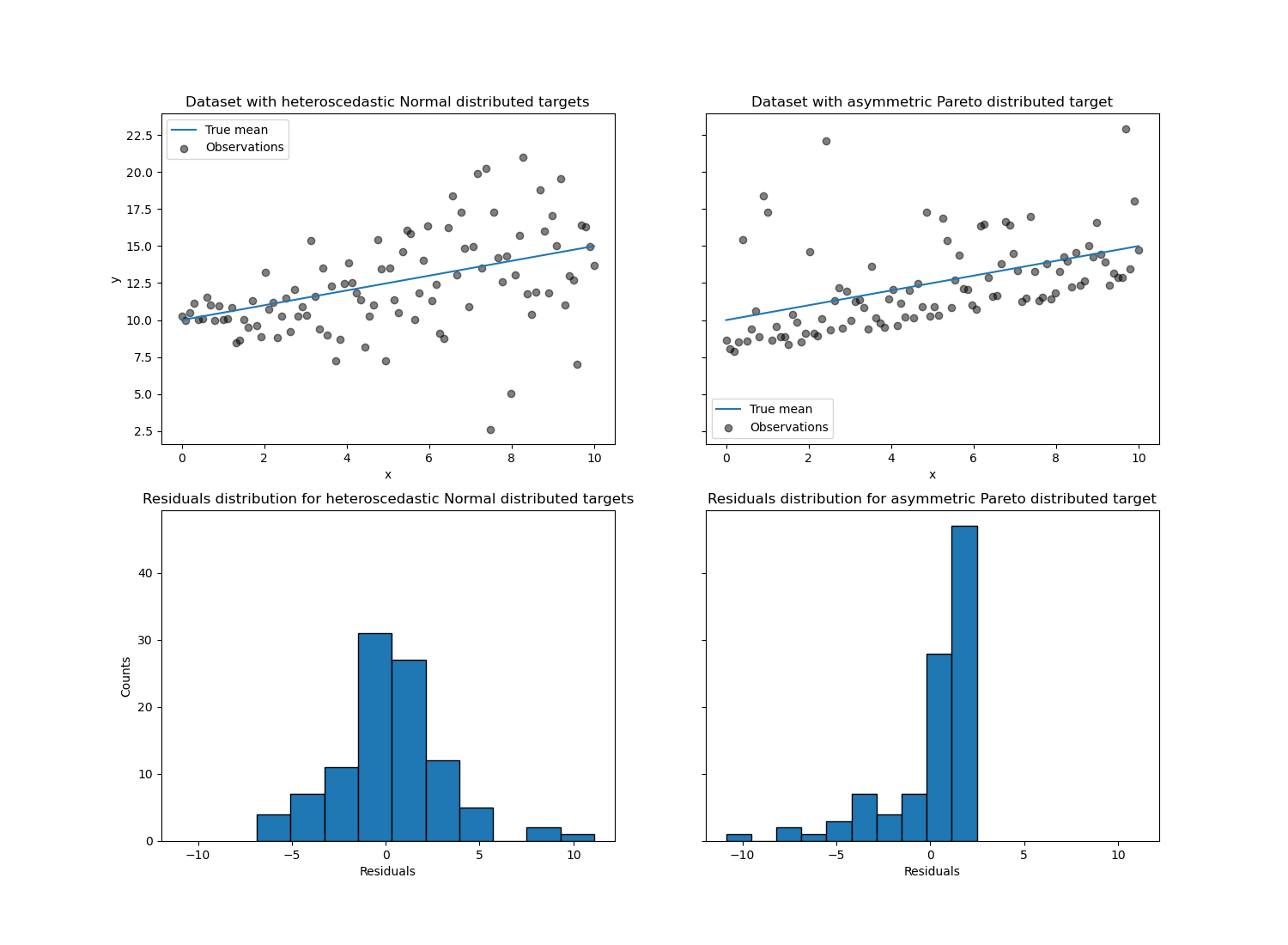
对于异方差正态分布的目标,我们观察到当特征 x 的值增加时,噪声的方差也随之增加。
对于非对称帕累托分布的目标,我们观察到正残差是有界的。
这类带噪声的目标使得通过 LinearRegression 进行估计的效率较低,即我们需要更多数据才能获得稳定的结果,此外,大的异常值可能对拟合系数产生巨大影响。(换句话说:在方差恒定的情况下,普通最小二乘估计器会随着样本量的增加而更快地收敛到真实系数。)
在这种非对称设置中,中位数或不同的分位数提供了额外的洞察力。最重要的是,中位数估计对异常值和重尾分布更加稳健。但请注意,极端分位数是由非常少的数据点估计的。95% 分位数或多或少是由前 5% 的最大值估计的,因此对异常值也有些敏感。
在本教程的其余部分,我们将展示 QuantileRegressor 如何在实践中使用,并提供对拟合模型属性的直观理解。最后,我们将比较 QuantileRegressor 和 LinearRegression。
拟合 QuantileRegressor#
在本节中,我们希望估计条件中位数以及分别固定在 5% 和 95% 的低分位数和高分位数。因此,我们将得到三个线性模型,每个分位数一个。
我们将使用 5% 和 95% 的分位数来查找训练样本中超出中心 90% 区间的异常值。
from sklearn.linear_model import QuantileRegressor

quantiles = [0.05, 0.5, 0.95]
predictions = {}
out_bounds_predictions = np.zeros_like(y_true_mean, dtype=np.bool_)
for quantile in quantiles:
    qr = QuantileRegressor(quantile=quantile, alpha=0)
    y_pred = qr.fit(X, y_normal).predict(X)
    predictions[quantile] = y_pred

    if quantile == min(quantiles):
        out_bounds_predictions = np.logical_or(
            out_bounds_predictions, y_pred >= y_normal
        )
    elif quantile == max(quantiles):
        out_bounds_predictions = np.logical_or(
            out_bounds_predictions, y_pred <= y_normal
        )
现在,我们可以绘制这三个线性模型,以及区分出位于中心 90% 区间内的样本和在此区间外的样本。
plt.plot(X, y_true_mean, color="black", linestyle="dashed", label="True mean")

for quantile, y_pred in predictions.items():
    plt.plot(X, y_pred, label=f"Quantile: {quantile}")

plt.scatter(
    x[out_bounds_predictions],
    y_normal[out_bounds_predictions],
    color="black",
    marker="+",
    alpha=0.5,
    label="Outside interval",
)
plt.scatter(
    x[~out_bounds_predictions],
    y_normal[~out_bounds_predictions],
    color="black",
    alpha=0.5,
    label="Inside interval",
)

plt.legend()
plt.xlabel("x")
plt.ylabel("y")
_ = plt.title("Quantiles of heteroscedastic Normal distributed target")
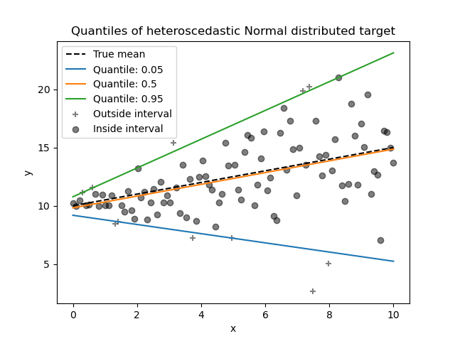
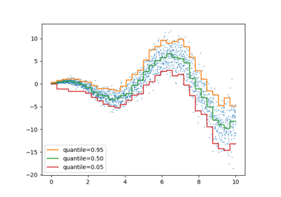
由于噪声仍然是正态分布,特别是对称的,因此真实的条件均值和真实的条件中位数是重合的。事实上,我们看到估计的中位数几乎达到了真实的均值。我们观察到噪声方差增加对 5% 和 95% 分位数的影响:这些分位数的斜率非常不同,并且随着 x 的增加,它们之间的区间变得更宽。
为了进一步直观理解 5% 和 95% 分位数估计器的含义,可以计算预测分位数(在上述图表中以交叉表示)之上和之下的样本数量,考虑到我们总共有 100 个样本。
我们可以使用非对称帕累托分布的目标重复相同的实验。
quantiles = [0.05, 0.5, 0.95]
predictions = {}
out_bounds_predictions = np.zeros_like(y_true_mean, dtype=np.bool_)
for quantile in quantiles:
    qr = QuantileRegressor(quantile=quantile, alpha=0)
    y_pred = qr.fit(X, y_pareto).predict(X)
    predictions[quantile] = y_pred

    if quantile == min(quantiles):
        out_bounds_predictions = np.logical_or(
            out_bounds_predictions, y_pred >= y_pareto
        )
    elif quantile == max(quantiles):
        out_bounds_predictions = np.logical_or(
            out_bounds_predictions, y_pred <= y_pareto
        )
plt.plot(X, y_true_mean, color="black", linestyle="dashed", label="True mean")

for quantile, y_pred in predictions.items():
    plt.plot(X, y_pred, label=f"Quantile: {quantile}")

plt.scatter(
    x[out_bounds_predictions],
    y_pareto[out_bounds_predictions],
    color="black",
    marker="+",
    alpha=0.5,
    label="Outside interval",
)
plt.scatter(
    x[~out_bounds_predictions],
    y_pareto[~out_bounds_predictions],
    color="black",
    alpha=0.5,
    label="Inside interval",
)

plt.legend()
plt.xlabel("x")
plt.ylabel("y")
_ = plt.title("Quantiles of asymmetric Pareto distributed target")
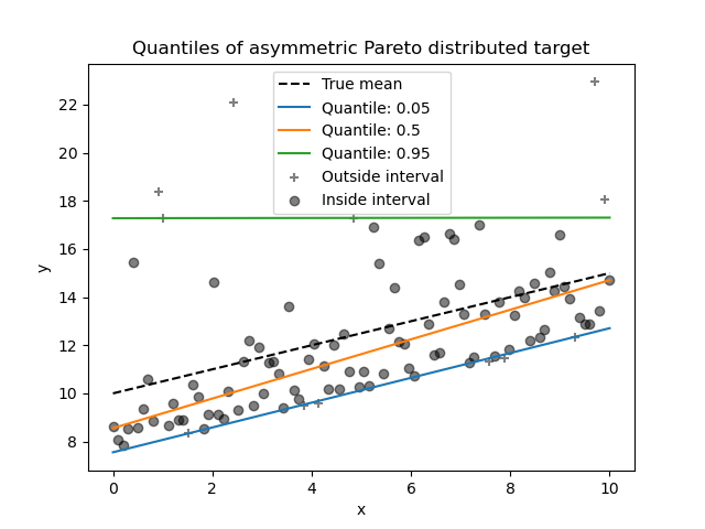
由于噪声分布的非对称性,我们观察到真实均值和估计的条件中位数是不同的。我们还观察到每个分位数模型都有不同的参数,以更好地拟合所需的分位数。请注意,理想情况下,在这种情况下所有分位数都将是平行的,这在有更多数据点或不那么极端的分位数(例如 10% 和 90%)时会变得更加明显。
比较 QuantileRegressor 和 LinearRegression#
在本节中,我们将重点讨论 QuantileRegressor 和 LinearRegression 最小化的损失函数之间的差异。
实际上,LinearRegression 是一种最小化训练目标和预测目标之间均方误差 (MSE) 的最小二乘方法。相比之下,QuantileRegressor 当 quantile=0.5 时,最小化的是平均绝对误差 (MAE)。
为什么这很重要?损失函数准确地指定了模型的目标预测内容,请参阅关于评分函数选择的用户指南。简而言之,最小化 MSE 的模型预测的是均值(期望),而最小化 MAE 的模型预测的是中位数。
让我们计算这些模型在均方误差和平均绝对误差方面的训练误差。我们将使用非对称帕累托分布的目标,以使其更有趣,因为均值和中位数不相等。
from sklearn.linear_model import LinearRegression
from sklearn.metrics import mean_absolute_error, mean_squared_error

linear_regression = LinearRegression()
quantile_regression = QuantileRegressor(quantile=0.5, alpha=0)

y_pred_lr = linear_regression.fit(X, y_pareto).predict(X)
y_pred_qr = quantile_regression.fit(X, y_pareto).predict(X)

print(
    "Training error (in-sample performance)\n"
    f"{'model':<20}   MAE   MSE\n"
    f"{linear_regression.__class__.__name__:<20} "
    f"{mean_absolute_error(y_pareto, y_pred_lr):5.3f} "
    f"{mean_squared_error(y_pareto, y_pred_lr):5.3f}\n"
    f"{quantile_regression.__class__.__name__:<20} "
    f"{mean_absolute_error(y_pareto, y_pred_qr):5.3f} "
    f"{mean_squared_error(y_pareto, y_pred_qr):5.3f}"
)
Training error (in-sample performance)
model                  MAE   MSE
LinearRegression     1.805 6.486
QuantileRegressor    1.670 7.025
在训练集上,我们看到 QuantileRegressor 的 MAE 低于 LinearRegression。相反,LinearRegression 的 MSE 低于 QuantileRegressor。这些结果证实了 MAE 是 QuantileRegressor 最小化的损失,而 MSE 是 LinearRegression 最小化的损失。
我们可以通过查看交叉验证获得的测试误差来进行类似的评估。
from sklearn.model_selection import cross_validate

cv_results_lr = cross_validate(
    linear_regression,
    X,
    y_pareto,
    cv=3,
    scoring=["neg_mean_absolute_error", "neg_mean_squared_error"],
)
cv_results_qr = cross_validate(
    quantile_regression,
    X,
    y_pareto,
    cv=3,
    scoring=["neg_mean_absolute_error", "neg_mean_squared_error"],
)
print(
    "Test error (cross-validated performance)\n"
    f"{'model':<20}   MAE   MSE\n"
    f"{linear_regression.__class__.__name__:<20} "
    f"{-cv_results_lr['test_neg_mean_absolute_error'].mean():5.3f} "
    f"{-cv_results_lr['test_neg_mean_squared_error'].mean():5.3f}\n"
    f"{quantile_regression.__class__.__name__:<20} "
    f"{-cv_results_qr['test_neg_mean_absolute_error'].mean():5.3f} "
    f"{-cv_results_qr['test_neg_mean_squared_error'].mean():5.3f}"
)
Test error (cross-validated performance)
model                  MAE   MSE
LinearRegression     1.732 6.690
QuantileRegressor    1.679 7.129
我们在样本外评估中得到了相似的结论。
脚本总运行时间: (0 分钟 0.870 秒)
相关示例