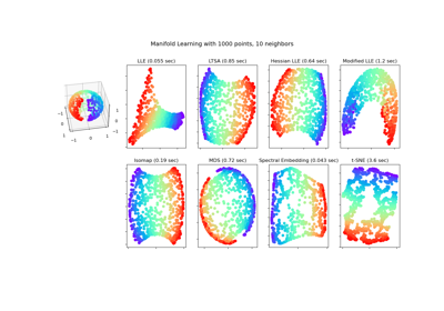
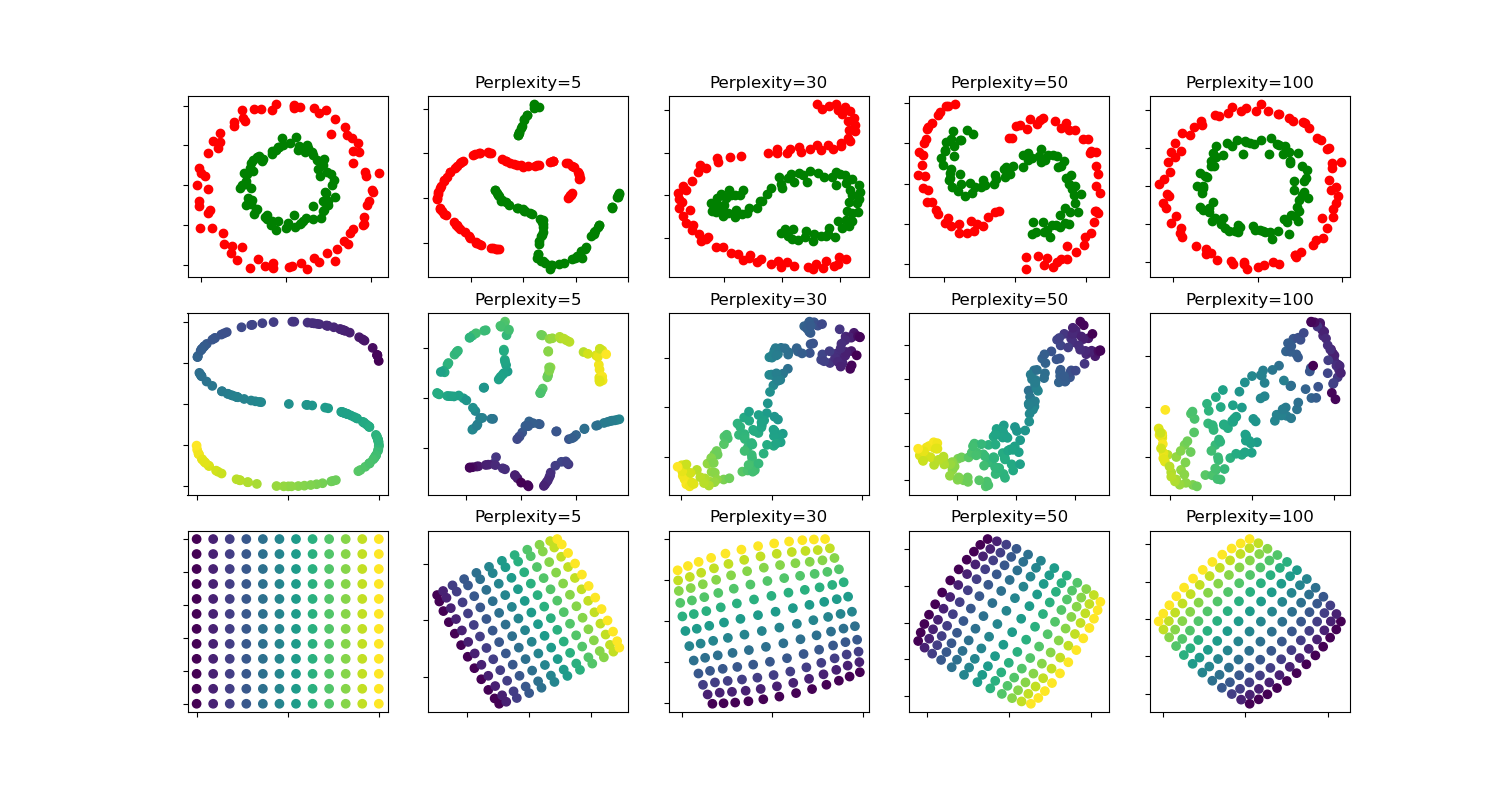
t-SNE：不同困惑度值对形状的影响#

t-SNE 在不同困惑度值下对两个同心圆和 S 形曲线数据集的效果演示。

我们观察到，随着困惑度值增加，形状趋于更清晰。

聚类的大小、距离和形状可能因初始化、困惑度值而异，并且不总是传达有意义的信息。

如下所示，t-SNE 在较高困惑度下能找到两个同心圆的有意义拓扑，但圆的大小和距离与原始略有不同。与两个同心圆数据集相反，在 S 形曲线数据集上，即使对于较大的困惑度值，其形状在视觉上仍偏离 S 形曲线拓扑。

更多详情，请参阅“如何有效使用 t-SNE” https://distill.pub/2016/misread-tsne/，其中对各种参数的影响进行了很好的讨论，并提供了交互式图表以探索这些影响。

Perplexity=5, Perplexity=30, Perplexity=50, Perplexity=100, Perplexity=5, Perplexity=30, Perplexity=50, Perplexity=100, Perplexity=5, Perplexity=30, Perplexity=50, Perplexity=100

circles, perplexity=5 in 0.13 sec
circles, perplexity=30 in 0.21 sec
circles, perplexity=50 in 0.23 sec
circles, perplexity=100 in 0.23 sec
S-curve, perplexity=5 in 0.13 sec
S-curve, perplexity=30 in 0.19 sec
S-curve, perplexity=50 in 0.23 sec
S-curve, perplexity=100 in 0.24 sec
uniform grid, perplexity=5 in 0.16 sec
uniform grid, perplexity=30 in 0.24 sec
uniform grid, perplexity=50 in 0.27 sec
uniform grid, perplexity=100 in 0.27 sec

# Authors: The scikit-learn developers
# SPDX-License-Identifier: BSD-3-Clause

from time import time

import matplotlib.pyplot as plt
import numpy as np
from matplotlib.ticker import NullFormatter

from sklearn import datasets, manifold

n_samples = 150
n_components = 2
(fig, subplots) = plt.subplots(3, 5, figsize=(15, 8))
perplexities = [5, 30, 50, 100]

X, y = datasets.make_circles(
    n_samples=n_samples, factor=0.5, noise=0.05, random_state=0
)

red = y == 0
green = y == 1

ax = subplots[0][0]
ax.scatter(X[red, 0], X[red, 1], c="r")
ax.scatter(X[green, 0], X[green, 1], c="g")
ax.xaxis.set_major_formatter(NullFormatter())
ax.yaxis.set_major_formatter(NullFormatter())
plt.axis("tight")

for i, perplexity in enumerate(perplexities):
    ax = subplots[0][i + 1]

    t0 = time()
    tsne = manifold.TSNE(
        n_components=n_components,
        init="random",
        random_state=0,
        perplexity=perplexity,
        max_iter=300,
    )
    Y = tsne.fit_transform(X)
    t1 = time()
    print("circles, perplexity=%d in %.2g sec" % (perplexity, t1 - t0))
    ax.set_title("Perplexity=%d" % perplexity)
    ax.scatter(Y[red, 0], Y[red, 1], c="r")
    ax.scatter(Y[green, 0], Y[green, 1], c="g")
    ax.xaxis.set_major_formatter(NullFormatter())
    ax.yaxis.set_major_formatter(NullFormatter())
    ax.axis("tight")

# Another example using s-curve
X, color = datasets.make_s_curve(n_samples, random_state=0)

ax = subplots[1][0]
ax.scatter(X[:, 0], X[:, 2], c=color)
ax.xaxis.set_major_formatter(NullFormatter())
ax.yaxis.set_major_formatter(NullFormatter())

for i, perplexity in enumerate(perplexities):
    ax = subplots[1][i + 1]

    t0 = time()
    tsne = manifold.TSNE(
        n_components=n_components,
        init="random",
        random_state=0,
        perplexity=perplexity,
        learning_rate="auto",
        max_iter=300,
    )
    Y = tsne.fit_transform(X)
    t1 = time()
    print("S-curve, perplexity=%d in %.2g sec" % (perplexity, t1 - t0))

    ax.set_title("Perplexity=%d" % perplexity)
    ax.scatter(Y[:, 0], Y[:, 1], c=color)
    ax.xaxis.set_major_formatter(NullFormatter())
    ax.yaxis.set_major_formatter(NullFormatter())
    ax.axis("tight")


# Another example using a 2D uniform grid
x = np.linspace(0, 1, int(np.sqrt(n_samples)))
xx, yy = np.meshgrid(x, x)
X = np.hstack(
    [
        xx.ravel().reshape(-1, 1),
        yy.ravel().reshape(-1, 1),
    ]
)
color = xx.ravel()
ax = subplots[2][0]
ax.scatter(X[:, 0], X[:, 1], c=color)
ax.xaxis.set_major_formatter(NullFormatter())
ax.yaxis.set_major_formatter(NullFormatter())

for i, perplexity in enumerate(perplexities):
    ax = subplots[2][i + 1]

    t0 = time()
    tsne = manifold.TSNE(
        n_components=n_components,
        init="random",
        random_state=0,
        perplexity=perplexity,
        max_iter=400,
    )
    Y = tsne.fit_transform(X)
    t1 = time()
    print("uniform grid, perplexity=%d in %.2g sec" % (perplexity, t1 - t0))

    ax.set_title("Perplexity=%d" % perplexity)
    ax.scatter(Y[:, 0], Y[:, 1], c=color)
    ax.xaxis.set_major_formatter(NullFormatter())
    ax.yaxis.set_major_formatter(NullFormatter())
    ax.axis("tight")


plt.show()

脚本总运行时间： (0 分 3.074 秒)

t-SNE：不同困惑度值对形状的影响#

本页