注意
跳转至末尾以下载完整示例代码,或通过 JupyterLite 或 Binder 在浏览器中运行此示例
scikit-learn 1.4 发布亮点#
我们很高兴地宣布 scikit-learn 1.4 发布!此版本增加了许多错误修复和改进,以及一些新的关键功能。下面我们详细介绍此版本的一些主要功能。有关所有更改的详尽列表,请参阅发布说明。
要安装最新版本(使用 pip)
pip install --upgrade scikit-learn
或使用 conda
conda install -c conda-forge scikit-learn
HistGradientBoosting 原生支持 DataFrame 中的类别 DType#
ensemble.HistGradientBoostingClassifier 和 ensemble.HistGradientBoostingRegressor 现在直接支持包含类别特征的 DataFrame。这里我们有一个包含类别和数值特征混合的数据集
from sklearn.datasets import fetch_openml

X_adult, y_adult = fetch_openml("adult", version=2, return_X_y=True)

# Remove redundant and non-feature columns
X_adult = X_adult.drop(["education-num", "fnlwgt"], axis="columns")
X_adult.dtypes
age                  int64
workclass         category
education         category
marital-status    category
occupation        category
relationship      category
race              category
sex               category
capital-gain         int64
capital-loss         int64
hours-per-week       int64
native-country    category
dtype: object
通过设置 categorical_features="from_dtype",梯度提升分类器将具有类别 dtype 的列视为算法中的类别特征
from sklearn.ensemble import HistGradientBoostingClassifier
from sklearn.metrics import roc_auc_score
from sklearn.model_selection import train_test_split

X_train, X_test, y_train, y_test = train_test_split(X_adult, y_adult, random_state=0)
hist = HistGradientBoostingClassifier(categorical_features="from_dtype")

hist.fit(X_train, y_train)
y_decision = hist.decision_function(X_test)
print(f"ROC AUC score is {roc_auc_score(y_test, y_decision)}")
ROC AUC score is 0.9282151413918491
set_output 中的 Polars 输出#
scikit-learn 的转换器现在支持使用 set_output API 的 Polars 输出。
import polars as pl

from sklearn.compose import ColumnTransformer
from sklearn.preprocessing import OneHotEncoder, StandardScaler

df = pl.DataFrame(
    {"height": [120, 140, 150, 110, 100], "pet": ["dog", "cat", "dog", "cat", "cat"]}
)
preprocessor = ColumnTransformer(
    [
        ("numerical", StandardScaler(), ["height"]),
        ("categorical", OneHotEncoder(sparse_output=False), ["pet"]),
    ],
    verbose_feature_names_out=False,
)
preprocessor.set_output(transform="polars")

df_out = preprocessor.fit_transform(df)
df_out
print(f"Output type: {type(df_out)}")
Output type: <class 'polars.dataframe.frame.DataFrame'>
随机森林的缺失值支持#
类 ensemble.RandomForestClassifier 和 ensemble.RandomForestRegressor 现在支持缺失值。在训练每个单独的树时,分割器会评估每个潜在的阈值,其中缺失值将分别分到左节点和右节点。更多详细信息请参阅用户指南。
import numpy as np

from sklearn.ensemble import RandomForestClassifier

X = np.array([0, 1, 6, np.nan]).reshape(-1, 1)
y = [0, 0, 1, 1]

forest = RandomForestClassifier(random_state=0).fit(X, y)
forest.predict(X)
array([0, 0, 1, 1])
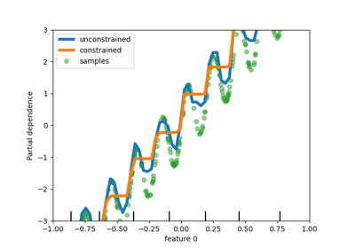
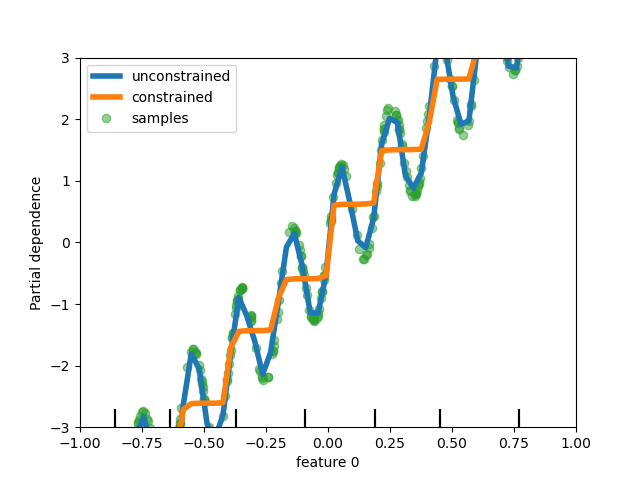
在基于树的模型中添加对单调约束的支持#
虽然我们已经在 scikit-learn 0.23 中添加了对基于直方图的梯度提升中单调约束的支持,但现在我们为所有其他基于树的模型(如决策树、随机森林、极端随机树和精确梯度提升)都支持此功能。这里,我们展示了随机森林在回归问题上的此功能。
import matplotlib.pyplot as plt

from sklearn.ensemble import RandomForestRegressor
from sklearn.inspection import PartialDependenceDisplay

n_samples = 500
rng = np.random.RandomState(0)
X = rng.randn(n_samples, 2)
noise = rng.normal(loc=0.0, scale=0.01, size=n_samples)
y = 5 * X[:, 0] + np.sin(10 * np.pi * X[:, 0]) - noise

rf_no_cst = RandomForestRegressor().fit(X, y)
rf_cst = RandomForestRegressor(monotonic_cst=[1, 0]).fit(X, y)

disp = PartialDependenceDisplay.from_estimator(
    rf_no_cst,
    X,
    features=[0],
    feature_names=["feature 0"],
    line_kw={"linewidth": 4, "label": "unconstrained", "color": "tab:blue"},
)
PartialDependenceDisplay.from_estimator(
    rf_cst,
    X,
    features=[0],
    line_kw={"linewidth": 4, "label": "constrained", "color": "tab:orange"},
    ax=disp.axes_,
)
disp.axes_[0, 0].plot(
    X[:, 0], y, "o", alpha=0.5, zorder=-1, label="samples", color="tab:green"
)
disp.axes_[0, 0].set_ylim(-3, 3)
disp.axes_[0, 0].set_xlim(-1, 1)
disp.axes_[0, 0].legend()
plt.show()
丰富的估计器显示#
估计器显示已得到丰富:如果我们查看上面定义的 forest
forest
通过点击图表右上角的“?”图标,可以访问估计器的文档。
此外,当估计器拟合后,显示颜色会从橙色变为蓝色。您也可以通过将鼠标悬停在“i”图标上来获取此信息。
from sklearn.base import clone

clone(forest)  # the clone is not fitted
元数据路由支持#
许多元估计器和交叉验证例程现在支持元数据路由,这些都在用户指南中列出。例如,您可以使用样本权重和 GroupKFold 进行嵌套交叉验证。
import sklearn
from sklearn.datasets import make_regression
from sklearn.linear_model import Lasso
from sklearn.metrics import get_scorer
from sklearn.model_selection import GridSearchCV, GroupKFold, cross_validate

# For now by default metadata routing is disabled, and need to be explicitly
# enabled.
sklearn.set_config(enable_metadata_routing=True)

n_samples = 100
X, y = make_regression(n_samples=n_samples, n_features=5, noise=0.5)
rng = np.random.RandomState(7)
groups = rng.randint(0, 10, size=n_samples)
sample_weights = rng.rand(n_samples)
estimator = Lasso().set_fit_request(sample_weight=True)
hyperparameter_grid = {"alpha": [0.1, 0.5, 1.0, 2.0]}
scoring_inner_cv = get_scorer("neg_mean_squared_error").set_score_request(
    sample_weight=True
)
inner_cv = GroupKFold(n_splits=5)

grid_search = GridSearchCV(
    estimator=estimator,
    param_grid=hyperparameter_grid,
    cv=inner_cv,
    scoring=scoring_inner_cv,
)

outer_cv = GroupKFold(n_splits=5)
scorers = {
    "mse": get_scorer("neg_mean_squared_error").set_score_request(sample_weight=True)
}
results = cross_validate(
    grid_search,
    X,
    y,
    cv=outer_cv,
    scoring=scorers,
    return_estimator=True,
    params={"sample_weight": sample_weights, "groups": groups},
)
print("cv error on test sets:", results["test_mse"])

# Setting the flag to the default `False` to avoid interference with other
# scripts.
sklearn.set_config(enable_metadata_routing=False)
cv error on test sets: [-0.32494606 -0.55423887 -0.18175828 -0.41730889 -0.30546994]
稀疏数据上 PCA 的内存和运行时效率提升#
PCA 现在能够通过利用 scipy.sparse.linalg.LinearOperator 为 arpack 求解器原生处理稀疏矩阵,从而避免在执行数据集协方差矩阵的特征值分解时实例化大型稀疏矩阵。
from time import time

import scipy.sparse as sp

from sklearn.decomposition import PCA

X_sparse = sp.random(m=1000, n=1000, random_state=0)
X_dense = X_sparse.toarray()

t0 = time()
PCA(n_components=10, svd_solver="arpack").fit(X_sparse)
time_sparse = time() - t0

t0 = time()
PCA(n_components=10, svd_solver="arpack").fit(X_dense)
time_dense = time() - t0

print(f"Speedup: {time_dense / time_sparse:.1f}x")
Speedup: 3.8x
脚本总运行时间: (0 分 2.225 秒)
相关示例