多项式和样条插值#

本示例演示如何使用岭回归通过高达 degree 次的多项式来近似一个函数。我们展示了给定 n_samples 个一维点 x_i 的两种不同方法：

PolynomialFeatures 生成高达 degree 次的所有单项式。这给了我们所谓的范德蒙矩阵，该矩阵有 n_samples 行和 degree + 1 列。
```
[[1, x_0, x_0 ** 2, x_0 ** 3, ..., x_0 ** degree],
 [1, x_1, x_1 ** 2, x_1 ** 3, ..., x_1 ** degree],
 ...]
```
直观地，该矩阵可以被解释为伪特征矩阵（点的值提升到某个幂次）。该矩阵类似于（但不同于）由多项式核引起的矩阵。
SplineTransformer 生成 B 样条基函数。B 样条的基函数是 degree 次的分段多项式函数，仅在 degree+1 个连续结点之间非零。给定 n_knots 个结点，这将产生一个矩阵，该矩阵有 n_samples 行和 n_knots + degree - 1 列。
```
[[basis_1(x_0), basis_2(x_0), ...],
 [basis_1(x_1), basis_2(x_1), ...],
 ...]
```

本示例展示了这两种转换器非常适合使用线性模型和通过管道添加非线性特征来建模非线性效应。核方法扩展了这一思想，可以引入非常高（甚至无限）维的特征空间。

# Authors: The scikit-learn developers
# SPDX-License-Identifier: BSD-3-Clause

import matplotlib.pyplot as plt
import numpy as np

from sklearn.linear_model import Ridge
from sklearn.pipeline import make_pipeline
from sklearn.preprocessing import PolynomialFeatures, SplineTransformer

我们首先定义一个打算近似的函数并准备绘制它。

def f(x):
    """Function to be approximated by polynomial interpolation."""
    return x * np.sin(x)


# whole range we want to plot
x_plot = np.linspace(-1, 11, 100)

为了使其有趣，我们只提供一小部分点进行训练。

x_train = np.linspace(0, 10, 100)
rng = np.random.RandomState(0)
x_train = np.sort(rng.choice(x_train, size=20, replace=False))
y_train = f(x_train)

# create 2D-array versions of these arrays to feed to transformers
X_train = x_train[:, np.newaxis]
X_plot = x_plot[:, np.newaxis]

现在我们准备创建多项式特征和样条，在训练点上进行拟合，并展示它们插值的效果。

# plot function
lw = 2
fig, ax = plt.subplots()
ax.set_prop_cycle(
    color=["black", "teal", "yellowgreen", "gold", "darkorange", "tomato"]
)
ax.plot(x_plot, f(x_plot), linewidth=lw, label="ground truth")

# plot training points
ax.scatter(x_train, y_train, label="training points")

# polynomial features
for degree in [3, 4, 5]:
    model = make_pipeline(PolynomialFeatures(degree), Ridge(alpha=1e-3))
    model.fit(X_train, y_train)
    y_plot = model.predict(X_plot)
    ax.plot(x_plot, y_plot, label=f"degree {degree}")

# B-spline with 4 + 3 - 1 = 6 basis functions
model = make_pipeline(SplineTransformer(n_knots=4, degree=3), Ridge(alpha=1e-3))
model.fit(X_train, y_train)

y_plot = model.predict(X_plot)
ax.plot(x_plot, y_plot, label="B-spline")
ax.legend(loc="lower center")
ax.set_ylim(-20, 10)
plt.show()

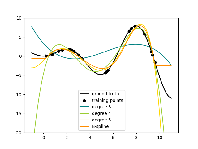
这很好地表明，更高次的多项式可以更好地拟合数据。但同时，过高的幂次可能会表现出不希望的振荡行为，并且对于拟合数据范围之外的外推尤其危险。这是 B 样条的一个优点。它们通常能像多项式一样很好地拟合数据，并表现出非常漂亮和平滑的行为。它们还具有很好的选项来控制外推，默认情况下是保持常数。请注意，通常情况下，您会增加结点的数量，但保持 degree=3。

为了更深入地了解生成的特征基，我们分别绘制了两个转换器的所有列。

fig, axes = plt.subplots(ncols=2, figsize=(16, 5))
pft = PolynomialFeatures(degree=3).fit(X_train)
axes[0].plot(x_plot, pft.transform(X_plot))
axes[0].legend(axes[0].lines, [f"degree {n}" for n in range(4)])
axes[0].set_title("PolynomialFeatures")

splt = SplineTransformer(n_knots=4, degree=3).fit(X_train)
axes[1].plot(x_plot, splt.transform(X_plot))
axes[1].legend(axes[1].lines, [f"spline {n}" for n in range(6)])
axes[1].set_title("SplineTransformer")

# plot knots of spline
knots = splt.bsplines_[0].t
axes[1].vlines(knots[3:-3], ymin=0, ymax=0.8, linestyles="dashed")
plt.show()

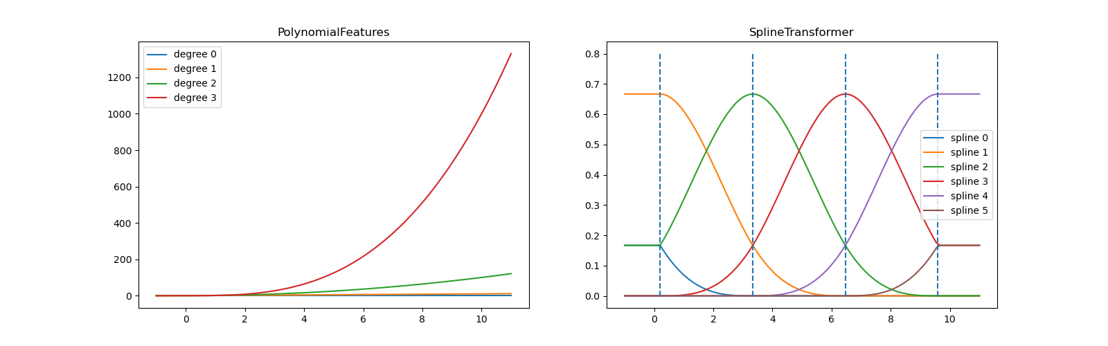
在左图中，我们识别出对应于从 x**0 到 x**3 的简单单项式的线条。在右图中，我们看到了 degree=3 的六个 B 样条基函数，以及在 fit 期间选择的四个结点位置。请注意，在拟合区间的左侧和右侧各有 degree 个额外的结点。这些结点是出于技术原因而存在的，因此我们不予显示。每个基函数都具有局部支持，并在拟合范围之外以常数形式延续。这种外推行为可以通过参数 extrapolation 进行更改。

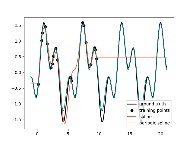
周期样条#

在前面的示例中，我们看到了多项式和样条在训练观测范围之外进行外推的局限性。在某些情况下，例如具有季节性效应时，我们期望底层信号是周期性延续的。这种效应可以使用周期样条进行建模，其在第一个和最后一个结点处具有相等函数值和相等导数。在下面的例子中，我们展示了周期样条如何在给定周期性附加信息的情况下，在训练数据范围内和范围之外提供更好的拟合。样条周期是第一个和最后一个结点之间的距离，我们手动指定该距离。

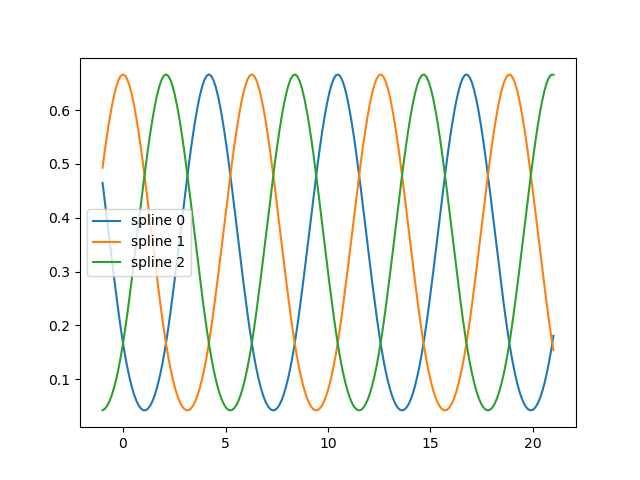
周期样条对于自然周期性特征（如一年中的某一天）也很有用，因为边界结点的平滑性可以防止转换值出现跳跃（例如从 12 月 31 日到 1 月 1 日）。对于此类自然周期性特征或更一般的已知周期特征，建议通过手动设置结点将此信息明确传递给 SplineTransformer。

def g(x):
    """Function to be approximated by periodic spline interpolation."""
    return np.sin(x) - 0.7 * np.cos(x * 3)


y_train = g(x_train)

# Extend the test data into the future:
x_plot_ext = np.linspace(-1, 21, 200)
X_plot_ext = x_plot_ext[:, np.newaxis]

lw = 2
fig, ax = plt.subplots()
ax.set_prop_cycle(color=["black", "tomato", "teal"])
ax.plot(x_plot_ext, g(x_plot_ext), linewidth=lw, label="ground truth")
ax.scatter(x_train, y_train, label="training points")

for transformer, label in [
    (SplineTransformer(degree=3, n_knots=10), "spline"),
    (
        SplineTransformer(
            degree=3,
            knots=np.linspace(0, 2 * np.pi, 10)[:, None],
            extrapolation="periodic",
        ),
        "periodic spline",
    ),
]:
    model = make_pipeline(transformer, Ridge(alpha=1e-3))
    model.fit(X_train, y_train)
    y_plot_ext = model.predict(X_plot_ext)
    ax.plot(x_plot_ext, y_plot_ext, label=label)

ax.legend()
fig.show()

fig, ax = plt.subplots()
knots = np.linspace(0, 2 * np.pi, 4)
splt = SplineTransformer(knots=knots[:, None], degree=3, extrapolation="periodic").fit(
    X_train
)
ax.plot(x_plot_ext, splt.transform(X_plot_ext))
ax.legend(ax.lines, [f"spline {n}" for n in range(3)])
plt.show()

脚本总运行时间： (0 分钟 0.423 秒)

多项式和样条插值#

周期样条#

此页