SVC 的正则化参数缩放#

以下示例说明了在使用支持向量机进行分类时，缩放正则化参数的效果。对于 SVC 分类，我们关注的是以下方程的风险最小化

\[C \sum_{i=1, n} \mathcal{L} (f(x_i), y_i) + \Omega (w)\]

其中

\(C\) 用于设置正则化量
\(\mathcal{L}\) 是我们样本和模型参数的损失函数。
\(\Omega\) 是我们模型参数的惩罚函数

如果我们将损失函数视为每个样本的个体误差，那么数据拟合项（即每个样本的误差总和）会随着样本数量的增加而增加。然而，惩罚项不会增加。

例如，当使用交叉验证来设置 C 的正则化量时，主问题与交叉验证折叠中的子问题之间会存在不同的样本数量。

由于损失函数依赖于样本数量，后者会影响 C 的选择值。由此产生的问题是“我们如何最优地调整 C 以适应不同数量的训练样本？”

# Authors: The scikit-learn developers
# SPDX-License-Identifier: BSD-3-Clause

数据生成#

在此示例中，我们探讨了在使用 L1 或 L2 惩罚时，重新参数化正则化参数 C 以考虑样本数量的效果。为此，我们创建了一个具有大量特征的合成数据集，其中只有少数特征是信息丰富的。因此，我们期望正则化将系数收缩到零（L2 惩罚）或恰好为零（L1 惩罚）。

from sklearn.datasets import make_classification

n_samples, n_features = 100, 300
X, y = make_classification(
    n_samples=n_samples, n_features=n_features, n_informative=5, random_state=1
)

L1 惩罚情况#

在 L1 情况下，理论指出，在强正则化下，估计器无法像已知真实分布的模型那样进行预测（即使在样本量趋于无穷大的极限情况下），因为它可能将一些原本具有预测性的特征权重设置为零，从而引入偏差。但是，它确实指出，通过调整 C，可以找到正确的非零参数集及其符号。

我们定义一个带有 L1 惩罚的线性 SVC。

from sklearn.svm import LinearSVC

model_l1 = LinearSVC(penalty="l1", loss="squared_hinge", dual=False, tol=1e-3)

我们通过交叉验证计算不同 C 值下的平均测试得分。

import numpy as np
import pandas as pd

from sklearn.model_selection import ShuffleSplit, validation_curve

Cs = np.logspace(-2.3, -1.3, 10)
train_sizes = np.linspace(0.3, 0.7, 3)
labels = [f"fraction: {train_size}" for train_size in train_sizes]
shuffle_params = {
    "test_size": 0.3,
    "n_splits": 150,
    "random_state": 1,
}

results = {"C": Cs}
for label, train_size in zip(labels, train_sizes):
    cv = ShuffleSplit(train_size=train_size, **shuffle_params)
    train_scores, test_scores = validation_curve(
        model_l1,
        X,
        y,
        param_name="C",
        param_range=Cs,
        cv=cv,
        n_jobs=2,
    )
    results[label] = test_scores.mean(axis=1)
results = pd.DataFrame(results)

import matplotlib.pyplot as plt

fig, axes = plt.subplots(nrows=1, ncols=2, sharey=True, figsize=(12, 6))

# plot results without scaling C
results.plot(x="C", ax=axes[0], logx=True)
axes[0].set_ylabel("CV score")
axes[0].set_title("No scaling")

for label in labels:
    best_C = results.loc[results[label].idxmax(), "C"]
    axes[0].axvline(x=best_C, linestyle="--", color="grey", alpha=0.7)

# plot results by scaling C
for train_size_idx, label in enumerate(labels):
    train_size = train_sizes[train_size_idx]
    results_scaled = results[[label]].assign(
        C_scaled=Cs * float(n_samples * np.sqrt(train_size))
    )
    results_scaled.plot(x="C_scaled", ax=axes[1], logx=True, label=label)
    best_C_scaled = results_scaled["C_scaled"].loc[results[label].idxmax()]
    axes[1].axvline(x=best_C_scaled, linestyle="--", color="grey", alpha=0.7)

axes[1].set_title("Scaling C by sqrt(1 / n_samples)")

_ = fig.suptitle("Effect of scaling C with L1 penalty")

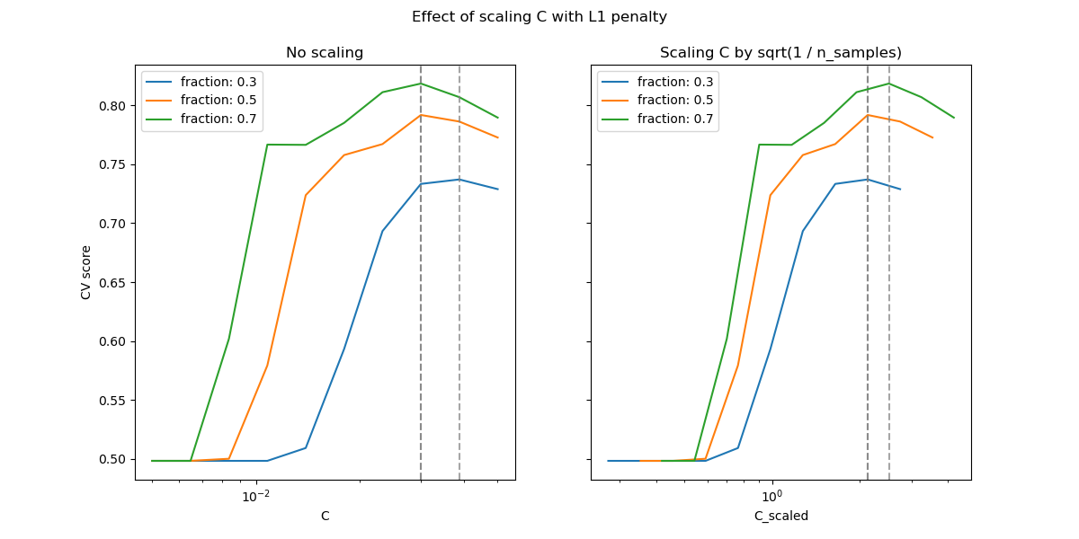
Effect of scaling C with L1 penalty, No scaling, Scaling C by sqrt(1 / n_samples)

在小 C 值区域（强正则化），模型学习到的所有系数都为零，导致严重的欠拟合。实际上，此区域的准确率处于随机水平。

使用默认缩放会导致 C 的最优值相对稳定，而脱离欠拟合区域的过渡则取决于训练样本的数量。重新参数化会带来更稳定的结果。

例如，请参阅 On the prediction performance of the Lasso 或 Simultaneous analysis of Lasso and Dantzig selector 的定理 3，其中正则化参数总是被假定与 1 / sqrt(n_samples) 成比例。

L2 惩罚情况#

我们可以用 L2 惩罚进行类似的实验。在这种情况下，理论指出，为了实现预测一致性，惩罚参数应随着样本数量的增加而保持不变。

model_l2 = LinearSVC(penalty="l2", loss="squared_hinge", dual=True)
Cs = np.logspace(-8, 4, 11)

labels = [f"fraction: {train_size}" for train_size in train_sizes]
results = {"C": Cs}
for label, train_size in zip(labels, train_sizes):
    cv = ShuffleSplit(train_size=train_size, **shuffle_params)
    train_scores, test_scores = validation_curve(
        model_l2,
        X,
        y,
        param_name="C",
        param_range=Cs,
        cv=cv,
        n_jobs=2,
    )
    results[label] = test_scores.mean(axis=1)
results = pd.DataFrame(results)

import matplotlib.pyplot as plt

fig, axes = plt.subplots(nrows=1, ncols=2, sharey=True, figsize=(12, 6))

# plot results without scaling C
results.plot(x="C", ax=axes[0], logx=True)
axes[0].set_ylabel("CV score")
axes[0].set_title("No scaling")

for label in labels:
    best_C = results.loc[results[label].idxmax(), "C"]
    axes[0].axvline(x=best_C, linestyle="--", color="grey", alpha=0.8)

# plot results by scaling C
for train_size_idx, label in enumerate(labels):
    results_scaled = results[[label]].assign(
        C_scaled=Cs * float(n_samples * np.sqrt(train_sizes[train_size_idx]))
    )
    results_scaled.plot(x="C_scaled", ax=axes[1], logx=True, label=label)
    best_C_scaled = results_scaled["C_scaled"].loc[results[label].idxmax()]
    axes[1].axvline(x=best_C_scaled, linestyle="--", color="grey", alpha=0.8)
axes[1].set_title("Scaling C by sqrt(1 / n_samples)")

fig.suptitle("Effect of scaling C with L2 penalty")
plt.show()

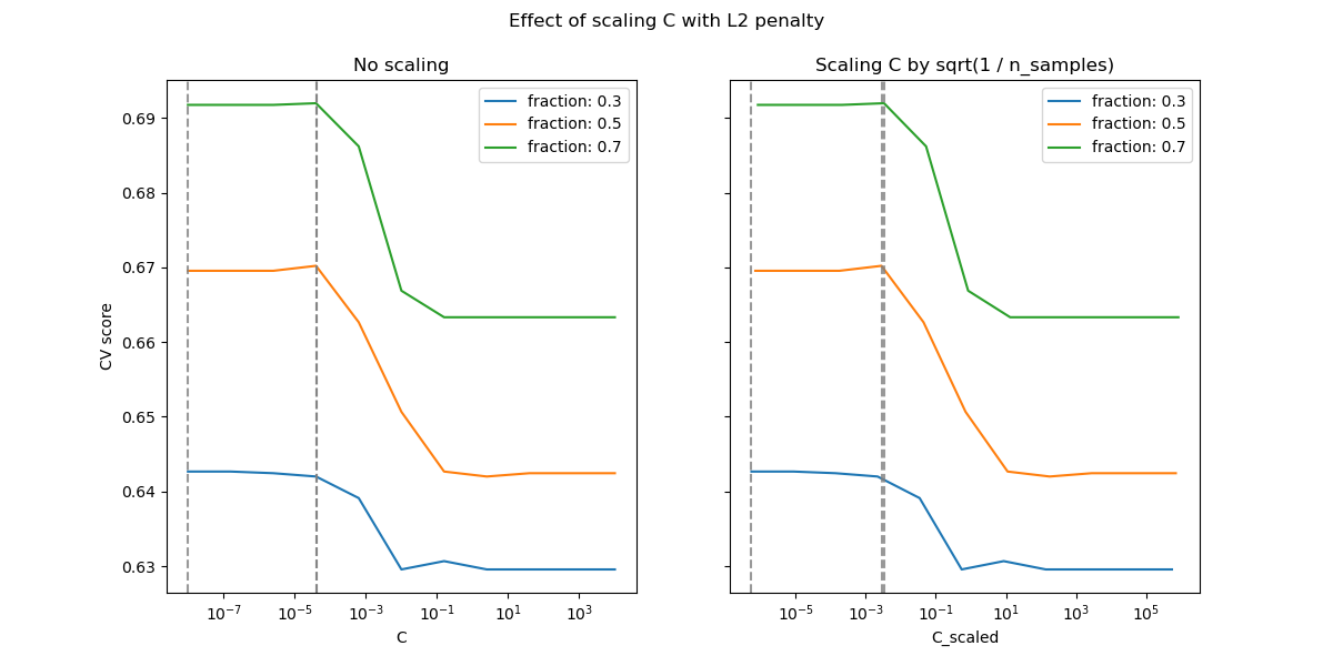
Effect of scaling C with L2 penalty, No scaling, Scaling C by sqrt(1 / n_samples)

对于 L2 惩罚情况，重新参数化对正则化最优值的稳定性影响较小。脱离过拟合区域的过渡发生在更广泛的范围内，并且准确率似乎没有降低到随机水平。

尝试将 n_splits=1_000 增加以在 L2 情况下获得更好的结果，由于文档构建器的限制，此处未显示。

脚本总运行时间： (0 分 17.612 秒)

SVC 的正则化参数缩放#

数据生成#

L1 惩罚情况#

L2 惩罚情况#

本页