鲁棒协方差估计与经验协方差估计对比

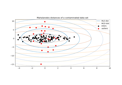
通常的协方差最大似然估计对数据集中的异常值非常敏感。在这种情况下，最好使用鲁棒协方差估计器，以确保估计结果对数据集中的“错误”观测值具有抵抗力。[1], [2]

最小协方差行列式估计器

最小协方差行列式估计器（Minimum Covariance Determinant，MCD）是一个鲁棒、高击穿点（即它可用于估计高度污染数据集的协方差矩阵，最多可处理\(\frac{n_\text{samples} - n_\text{features}-1}{2}\)个异常值）的协方差估计器。其思想是找到\(\frac{n_\text{samples} + n_\text{features}+1}{2}\)个观测值，其经验协方差具有最小行列式，从而得到一个“纯净”的观测值子集，并从该子集计算位置和协方差的标准估计。经过旨在补偿估计仅从初始数据一部分学习的事实校正步骤后，我们最终得到数据集位置和协方差的鲁棒估计。

最小协方差行列式估计器（MCD）由P.J.Rousseuw在[3]中提出。

评估

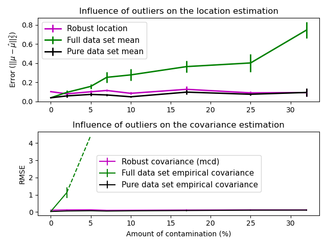
在此示例中，我们比较了在受污染的高斯分布数据集上使用各种类型的位置和协方差估计时所产生的估计误差

• 完整数据集的均值和经验协方差，它们在数据集中存在异常值时立即失效

• 鲁棒MCD，在\(n_\text{samples} > 5n_\text{features}\)的条件下误差较低

• 已知为良好观测值的均值和经验协方差。这可被视为“完美”的MCD估计，因此可以通过与此情况进行比较来信任我们的实现。

参考文献

[1]

Johanna Hardin, David M Rocke. The distribution of robust distances. Journal of Computational and Graphical Statistics. December 1, 2005, 14(4): 928-946.

[2]

Zoubir A., Koivunen V., Chakhchoukh Y. and Muma M. (2012). Robust estimation in signal processing: A tutorial-style treatment of fundamental concepts. IEEE Signal Processing Magazine 29(4), 61-80.

[3]

P. J. Rousseeuw. Least median of squares regression. Journal of American Statistical Ass., 79:871, 1984.

# Authors: The scikit-learn developers
# SPDX-License-Identifier: BSD-3-Clause

import matplotlib.font_manager
import matplotlib.pyplot as plt
import numpy as np

from sklearn.covariance import EmpiricalCovariance, MinCovDet

# example settings
n_samples = 80
n_features = 5
repeat = 10

range_n_outliers = np.concatenate(
    (
        np.linspace(0, n_samples / 8, 5),
        np.linspace(n_samples / 8, n_samples / 2, 5)[1:-1],
    )
).astype(int)

# definition of arrays to store results
err_loc_mcd = np.zeros((range_n_outliers.size, repeat))
err_cov_mcd = np.zeros((range_n_outliers.size, repeat))
err_loc_emp_full = np.zeros((range_n_outliers.size, repeat))
err_cov_emp_full = np.zeros((range_n_outliers.size, repeat))
err_loc_emp_pure = np.zeros((range_n_outliers.size, repeat))
err_cov_emp_pure = np.zeros((range_n_outliers.size, repeat))

# computation
for i, n_outliers in enumerate(range_n_outliers):
    for j in range(repeat):
        rng = np.random.RandomState(i * j)

        # generate data
        X = rng.randn(n_samples, n_features)
        # add some outliers
        outliers_index = rng.permutation(n_samples)[:n_outliers]
        outliers_offset = 10.0 * (
            np.random.randint(2, size=(n_outliers, n_features)) - 0.5
        )
        X[outliers_index] += outliers_offset
        inliers_mask = np.ones(n_samples).astype(bool)
        inliers_mask[outliers_index] = False

        # fit a Minimum Covariance Determinant (MCD) robust estimator to data
        mcd = MinCovDet().fit(X)
        # compare raw robust estimates with the true location and covariance
        err_loc_mcd[i, j] = np.sum(mcd.location_**2)
        err_cov_mcd[i, j] = mcd.error_norm(np.eye(n_features))

        # compare estimators learned from the full data set with true
        # parameters
        err_loc_emp_full[i, j] = np.sum(X.mean(0) ** 2)
        err_cov_emp_full[i, j] = (
            EmpiricalCovariance().fit(X).error_norm(np.eye(n_features))
        )

        # compare with an empirical covariance learned from a pure data set
        # (i.e. "perfect" mcd)
        pure_X = X[inliers_mask]
        pure_location = pure_X.mean(0)
        pure_emp_cov = EmpiricalCovariance().fit(pure_X)
        err_loc_emp_pure[i, j] = np.sum(pure_location**2)
        err_cov_emp_pure[i, j] = pure_emp_cov.error_norm(np.eye(n_features))

# Display results
font_prop = matplotlib.font_manager.FontProperties(size=11)
plt.subplot(2, 1, 1)
lw = 2
plt.errorbar(
    range_n_outliers,
    err_loc_mcd.mean(1),
    yerr=err_loc_mcd.std(1) / np.sqrt(repeat),
    label="Robust location",
    lw=lw,
    color="m",
)
plt.errorbar(
    range_n_outliers,
    err_loc_emp_full.mean(1),
    yerr=err_loc_emp_full.std(1) / np.sqrt(repeat),
    label="Full data set mean",
    lw=lw,
    color="green",
)
plt.errorbar(
    range_n_outliers,
    err_loc_emp_pure.mean(1),
    yerr=err_loc_emp_pure.std(1) / np.sqrt(repeat),
    label="Pure data set mean",
    lw=lw,
    color="black",
)
plt.title("Influence of outliers on the location estimation")
plt.ylabel(r"Error ($||\mu - \hat{\mu}||_2^2$)")
plt.legend(loc="upper left", prop=font_prop)

plt.subplot(2, 1, 2)
x_size = range_n_outliers.size
plt.errorbar(
    range_n_outliers,
    err_cov_mcd.mean(1),
    yerr=err_cov_mcd.std(1),
    label="Robust covariance (mcd)",
    color="m",
)
plt.errorbar(
    range_n_outliers[: (x_size // 5 + 1)],
    err_cov_emp_full.mean(1)[: (x_size // 5 + 1)],
    yerr=err_cov_emp_full.std(1)[: (x_size // 5 + 1)],
    label="Full data set empirical covariance",
    color="green",
)
plt.plot(
    range_n_outliers[(x_size // 5) : (x_size // 2 - 1)],
    err_cov_emp_full.mean(1)[(x_size // 5) : (x_size // 2 - 1)],
    color="green",
    ls="--",
)
plt.errorbar(
    range_n_outliers,
    err_cov_emp_pure.mean(1),
    yerr=err_cov_emp_pure.std(1),
    label="Pure data set empirical covariance",
    color="black",
)
plt.title("Influence of outliers on the covariance estimation")
plt.xlabel("Amount of contamination (%)")
plt.ylabel("RMSE")
plt.legend(loc="center", prop=font_prop)

plt.tight_layout()
plt.show()

相关示例

鲁棒协方差估计与马哈拉诺比斯距离的相关性

鲁棒协方差估计与马哈拉诺比斯距离的相关性

真实数据集上的异常值检测

真实数据集上的异常值检测

Ledoit-Wolf与OAS估计对比

Ledoit-Wolf与OAS估计对比

带协方差椭球的线性判别分析和二次判别分析

带协方差椭球的线性判别分析和二次判别分析