注意
转到末尾 下载完整的示例代码。或通过JupyterLite或Binder在浏览器中运行此示例
比较目标编码器与其他编码器#
TargetEncoder 使用目标值来编码每个类别特征。在此示例中,我们将比较处理类别特征的三种不同方法:TargetEncoder、OrdinalEncoder、OneHotEncoder 以及删除类别。
注意
fit(X, y).transform(X) 不等于 fit_transform(X, y),因为 fit_transform 中使用了交叉拟合方案进行编码。详见 用户指南。
# Authors: The scikit-learn developers
# SPDX-License-Identifier: BSD-3-Clause
从OpenML加载数据#
首先,我们加载葡萄酒评论数据集,其中目标是评论者给出的评分。
from sklearn.datasets import fetch_openml

wine_reviews = fetch_openml(data_id=42074, as_frame=True)

df = wine_reviews.frame
df.head()
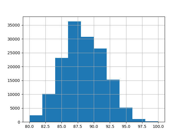
在此示例中,我们使用数据中数值和类别特征的以下子集。目标是80到100的连续值。
numerical_features = ["price"]
categorical_features = [
    "country",
    "province",
    "region_1",
    "region_2",
    "variety",
    "winery",
]
target_name = "points"

X = df[numerical_features + categorical_features]
y = df[target_name]

_ = y.hist()
使用不同编码器训练和评估管道#
在本节中,我们将使用不同编码策略评估带 HistGradientBoostingRegressor 的管道。首先,我们列出将用于预处理类别特征的编码器。
from sklearn.compose import ColumnTransformer
from sklearn.preprocessing import OneHotEncoder, OrdinalEncoder, TargetEncoder

categorical_preprocessors = [
    ("drop", "drop"),
    ("ordinal", OrdinalEncoder(handle_unknown="use_encoded_value", unknown_value=-1)),
    (
        "one_hot",
        OneHotEncoder(handle_unknown="ignore", max_categories=20, sparse_output=False),
    ),
    ("target", TargetEncoder(target_type="continuous")),
]
接下来,我们使用交叉验证评估模型并记录结果。
from sklearn.ensemble import HistGradientBoostingRegressor
from sklearn.model_selection import cross_validate
from sklearn.pipeline import make_pipeline

n_cv_folds = 3
max_iter = 20
results = []


def evaluate_model_and_store(name, pipe):
    result = cross_validate(
        pipe,
        X,
        y,
        scoring="neg_root_mean_squared_error",
        cv=n_cv_folds,
        return_train_score=True,
    )
    rmse_test_score = -result["test_score"]
    rmse_train_score = -result["train_score"]
    results.append(
        {
            "preprocessor": name,
            "rmse_test_mean": rmse_test_score.mean(),
            "rmse_test_std": rmse_train_score.std(),
            "rmse_train_mean": rmse_train_score.mean(),
            "rmse_train_std": rmse_train_score.std(),
        }
    )


for name, categorical_preprocessor in categorical_preprocessors:
    preprocessor = ColumnTransformer(
        [
            ("numerical", "passthrough", numerical_features),
            ("categorical", categorical_preprocessor, categorical_features),
        ]
    )
    pipe = make_pipeline(
        preprocessor, HistGradientBoostingRegressor(random_state=0, max_iter=max_iter)
    )
    evaluate_model_and_store(name, pipe)
原生类别特征支持#
在本节中,我们构建并评估一个使用 HistGradientBoostingRegressor 中原生类别特征支持的管道,该支持仅支持最多255个唯一类别。在我们的数据集中,大多数类别特征具有超过255个唯一类别。
n_unique_categories = df[categorical_features].nunique().sort_values(ascending=False)
n_unique_categories
winery      14810
region_1     1236
variety       632
province      455
country        48
region_2       18
dtype: int64
为了解决上述限制,我们将类别特征分为低基数和高基数特征。高基数特征将进行目标编码,而低基数特征将使用梯度提升中的原生类别特征。
high_cardinality_features = n_unique_categories[n_unique_categories > 255].index
low_cardinality_features = n_unique_categories[n_unique_categories <= 255].index
mixed_encoded_preprocessor = ColumnTransformer(
    [
        ("numerical", "passthrough", numerical_features),
        (
            "high_cardinality",
            TargetEncoder(target_type="continuous"),
            high_cardinality_features,
        ),
        (
            "low_cardinality",
            OrdinalEncoder(handle_unknown="use_encoded_value", unknown_value=-1),
            low_cardinality_features,
        ),
    ],
    verbose_feature_names_out=False,
)

# The output of the of the preprocessor must be set to pandas so the
# gradient boosting model can detect the low cardinality features.
mixed_encoded_preprocessor.set_output(transform="pandas")
mixed_pipe = make_pipeline(
    mixed_encoded_preprocessor,
    HistGradientBoostingRegressor(
        random_state=0, max_iter=max_iter, categorical_features=low_cardinality_features
    ),
)
mixed_pipe
Pipeline(steps=[('columntransformer',
                 ColumnTransformer(transformers=[('numerical', 'passthrough',
                                                  ['price']),
                                                 ('high_cardinality',
                                                  TargetEncoder(target_type='continuous'),
                                                  Index(['winery', 'region_1', 'variety', 'province'], dtype='object')),
                                                 ('low_cardinality',
                                                  OrdinalEncoder(handle_unknown='use_encoded_value',
                                                                 unknown_value=-1),
                                                  Index(['country', 'region_2'], dtype='object'))],
                                   verbose_feature_names_out=False)),
                ('histgradientboostingregressor',
                 HistGradientBoostingRegressor(categorical_features=Index(['country', 'region_2'], dtype='object'),
                                               max_iter=20, random_state=0))])
最后,我们使用交叉验证评估管道并记录结果。
evaluate_model_and_store("mixed_target", mixed_pipe)
绘制结果#
在本节中,我们通过绘制测试和训练分数来显示结果。
import matplotlib.pyplot as plt
import pandas as pd

results_df = (
    pd.DataFrame(results).set_index("preprocessor").sort_values("rmse_test_mean")
)

fig, (ax1, ax2) = plt.subplots(
    1, 2, figsize=(12, 8), sharey=True, constrained_layout=True
)
xticks = range(len(results_df))
name_to_color = dict(
    zip((r["preprocessor"] for r in results), ["C0", "C1", "C2", "C3", "C4"])
)

for subset, ax in zip(["test", "train"], [ax1, ax2]):
    mean, std = f"rmse_{subset}_mean", f"rmse_{subset}_std"
    data = results_df[[mean, std]].sort_values(mean)
    ax.bar(
        x=xticks,
        height=data[mean],
        yerr=data[std],
        width=0.9,
        color=[name_to_color[name] for name in data.index],
    )
    ax.set(
        title=f"RMSE ({subset.title()})",
        xlabel="Encoding Scheme",
        xticks=xticks,
        xticklabels=data.index,
    )
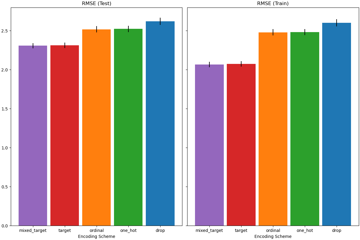
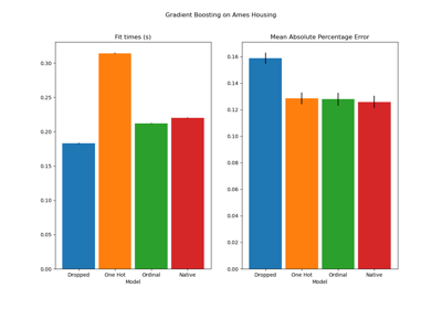
在评估测试集上的预测性能时,删除类别表现最差,而目标编码器表现最好。这可以解释如下:
删除类别特征使得管道的表达能力降低,从而导致欠拟合;
由于基数较高,为了减少训练时间,独热编码方案使用
max_categories=20,这限制了特征的过度扩展,可能导致欠拟合。如果我们没有设置
max_categories=20,独热编码方案很可能会使管道过拟合,因为特征数量会因与目标偶然相关(仅在训练集上)的稀有类别出现而爆炸;顺序编码对特征施加了任意顺序,然后
HistGradientBoostingRegressor将其视为数值。由于此模型将数值特征分组为每个特征256个 bin,许多不相关的类别可能会被分到一起,从而导致整个管道欠拟合;使用目标编码器时,会发生相同的分箱,但由于编码值在统计上按与目标变量的边际关联进行排序,
HistGradientBoostingRegressor使用的分箱变得有意义并带来了良好的结果:平滑目标编码和分箱的组合是一种很好的正则化策略,既能防止过拟合,又不过度限制管道的表达能力。
脚本总运行时间: (0 分钟 22.041 秒)
相关示例