注意
转到末尾 下载完整示例代码。或通过 JupyterLite 或 Binder 在浏览器中运行此示例
多类别接收者操作特征 (ROC)#
本示例介绍了如何使用接收者操作特征 (ROC) 指标来评估多类别分类器的质量。
ROC 曲线通常以真阳性率 (TPR) 为 Y 轴,假阳性率 (FPR) 为 X 轴。这意味着图表的左上角是“理想”点——FPR 为零,TPR 为一。这不是很现实,但它确实意味着曲线下面积 (AUC) 越大通常越好。ROC 曲线的“陡峭程度”也很重要,因为理想情况是最大化 TPR 同时最小化 FPR。
ROC 曲线通常用于二元分类,其中 TPR 和 FPR 可以明确定义。在多类别分类的情况下,只有在输出二值化后才能获得 TPR 或 FPR 的概念。这可以通过 2 种不同的方式完成
“一对多”方案将每个类别与所有其他类别(视为一个)进行比较;
“一对一”方案比较所有唯一的类别对组合。
在本示例中,我们探讨了这两种方案,并演示了微观平均和宏观平均的概念,作为总结多类别 ROC 曲线信息的不同方式。
注意
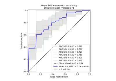
请参阅 带交叉验证的接收者操作特征 (ROC),以获取本示例的扩展,该扩展估算了 ROC 曲线及其各自 AUC 的方差。
# Authors: The scikit-learn developers
# SPDX-License-Identifier: BSD-3-Clause
加载和准备数据#
我们导入了 鸢尾花数据集,其中包含 3 个类别,每个类别对应一种鸢尾花类型。其中一个类别与另外两个类别是线性可分的;后两者之间是不可线性可分的。
在这里,我们对输出进行二值化,并添加噪声特征以增加问题的难度。
import numpy as np

from sklearn.datasets import load_iris
from sklearn.model_selection import train_test_split

iris = load_iris()
target_names = iris.target_names
X, y = iris.data, iris.target
y = iris.target_names[y]

random_state = np.random.RandomState(0)
n_samples, n_features = X.shape
n_classes = len(np.unique(y))
X = np.concatenate([X, random_state.randn(n_samples, 200 * n_features)], axis=1)
(
    X_train,
    X_test,
    y_train,
    y_test,
) = train_test_split(X, y, test_size=0.5, stratify=y, random_state=0)
我们训练了一个 LogisticRegression 模型,该模型由于使用了多项式公式,可以自然地处理多类别问题。
from sklearn.linear_model import LogisticRegression

classifier = LogisticRegression()
y_score = classifier.fit(X_train, y_train).predict_proba(X_test)
一对多 (One-vs-Rest) 多类别 ROC#
“一对多”(OvR) 多类别策略,也称为“一对全”,包括为每个 n_classes 计算一条 ROC 曲线。在每个步骤中,给定类别被视为正类别,其余类别被视为负类别。
注意
不应将用于评估多类别分类器的 OvR 策略与通过拟合一组二元分类器(例如通过 OneVsRestClassifier 元估计器)来训练多类别分类器的 OvR 策略混淆。OvR ROC 评估可用于检查任何类型的分类模型,无论其训练方式如何(请参阅 多类别和多输出算法)。
在本节中,我们使用 LabelBinarizer 以 OvR 方式通过独热编码对目标进行二值化。这意味着形状为 (n_samples,) 的目标被映射到形状为 (n_samples, n_classes) 的目标。
from sklearn.preprocessing import LabelBinarizer

label_binarizer = LabelBinarizer().fit(y_train)
y_onehot_test = label_binarizer.transform(y_test)
y_onehot_test.shape  # (n_samples, n_classes)
(75, 3)
我们也可以轻松检查特定类别的编码
label_binarizer.transform(["virginica"])
array([[0, 0, 1]])
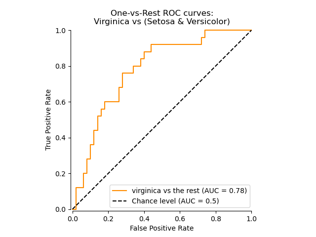
显示特定类别的 ROC 曲线#
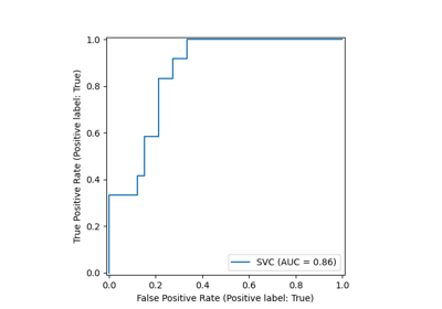
在下面的图中,我们展示了将鸢尾花视为“维吉尼亚鸢尾”(class_id=2)或“非维吉尼亚鸢尾”(其余)时的 ROC 曲线。
class_of_interest = "virginica"
class_id = np.flatnonzero(label_binarizer.classes_ == class_of_interest)[0]
class_id
np.int64(2)
import matplotlib.pyplot as plt

from sklearn.metrics import RocCurveDisplay

display = RocCurveDisplay.from_predictions(
    y_onehot_test[:, class_id],
    y_score[:, class_id],
    name=f"{class_of_interest} vs the rest",
    curve_kwargs=dict(color="darkorange"),
    plot_chance_level=True,
    despine=True,
)
_ = display.ax_.set(
    xlabel="False Positive Rate",
    ylabel="True Positive Rate",
    title="One-vs-Rest ROC curves:\nVirginica vs (Setosa & Versicolor)",
)
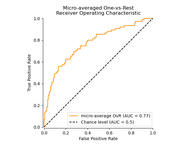
使用微观平均 OvR 的 ROC 曲线#
微观平均通过聚合所有类别的贡献(使用 numpy.ravel)来计算平均指标,如下所示
\(TPR=\frac{\sum_{c}TP_c}{\sum_{c}(TP_c + FN_c)}\) ;
\(FPR=\frac{\sum_{c}FP_c}{\sum_{c}(FP_c + TN_c)}\) .
我们可以简要演示 numpy.ravel 的效果
print(f"y_score:\n{y_score[0:2, :]}")
print()
print(f"y_score.ravel():\n{y_score[0:2, :].ravel()}")
y_score:
[[0.38 0.05 0.57]
 [0.07 0.28 0.65]]

y_score.ravel():
[0.38 0.05 0.57 0.07 0.28 0.65]
在类别高度不平衡的多类别分类设置中,微观平均优于宏观平均。在这种情况下,可以选择使用加权宏观平均,此处未作演示。
display = RocCurveDisplay.from_predictions(
    y_onehot_test.ravel(),
    y_score.ravel(),
    name="micro-average OvR",
    curve_kwargs=dict(color="darkorange"),
    plot_chance_level=True,
    despine=True,
)
_ = display.ax_.set(
    xlabel="False Positive Rate",
    ylabel="True Positive Rate",
    title="Micro-averaged One-vs-Rest\nReceiver Operating Characteristic",
)
如果主要关注的不是图表本身,而是 ROC-AUC 分数,我们可以使用 roc_auc_score 重现图中显示的值。
from sklearn.metrics import roc_auc_score

micro_roc_auc_ovr = roc_auc_score(
    y_test,
    y_score,
    multi_class="ovr",
    average="micro",
)

print(f"Micro-averaged One-vs-Rest ROC AUC score:\n{micro_roc_auc_ovr:.2f}")
Micro-averaged One-vs-Rest ROC AUC score:
0.77
这等同于使用 roc_curve 计算 ROC 曲线,然后使用 auc 计算展开的真实类别和预测类别的曲线下面积。
from sklearn.metrics import auc, roc_curve

# store the fpr, tpr, and roc_auc for all averaging strategies
fpr, tpr, roc_auc = dict(), dict(), dict()
# Compute micro-average ROC curve and ROC area
fpr["micro"], tpr["micro"], _ = roc_curve(y_onehot_test.ravel(), y_score.ravel())
roc_auc["micro"] = auc(fpr["micro"], tpr["micro"])

print(f"Micro-averaged One-vs-Rest ROC AUC score:\n{roc_auc['micro']:.2f}")
Micro-averaged One-vs-Rest ROC AUC score:
0.77
注意
默认情况下,ROC 曲线的计算通过使用线性插值和 McClish 校正 [ROC 曲线一部分的分析,医学决策制定。1989 年 7-9 月;9(3):190-5。],在最大假阳性率处添加一个点。
使用 OvR 宏观平均的 ROC 曲线#
获得宏观平均需要为每个类别独立计算指标,然后取其平均值,从而先验地平等对待所有类别。我们首先按类别汇总真阳性率/假阳性率
\(TPR=\frac{1}{C}\sum_{c}\frac{TP_c}{TP_c + FN_c}\) ;
\(FPR=\frac{1}{C}\sum_{c}\frac{FP_c}{FP_c + TN_c}\) .
其中 C 是类别的总数。
for i in range(n_classes):
    fpr[i], tpr[i], _ = roc_curve(y_onehot_test[:, i], y_score[:, i])
    roc_auc[i] = auc(fpr[i], tpr[i])

fpr_grid = np.linspace(0.0, 1.0, 1000)

# Interpolate all ROC curves at these points
mean_tpr = np.zeros_like(fpr_grid)

for i in range(n_classes):
    mean_tpr += np.interp(fpr_grid, fpr[i], tpr[i])  # linear interpolation

# Average it and compute AUC
mean_tpr /= n_classes

fpr["macro"] = fpr_grid
tpr["macro"] = mean_tpr
roc_auc["macro"] = auc(fpr["macro"], tpr["macro"])

print(f"Macro-averaged One-vs-Rest ROC AUC score:\n{roc_auc['macro']:.2f}")
Macro-averaged One-vs-Rest ROC AUC score:
0.78
此计算等同于简单调用
macro_roc_auc_ovr = roc_auc_score(
    y_test,
    y_score,
    multi_class="ovr",
    average="macro",
)

print(f"Macro-averaged One-vs-Rest ROC AUC score:\n{macro_roc_auc_ovr:.2f}")
Macro-averaged One-vs-Rest ROC AUC score:
0.78
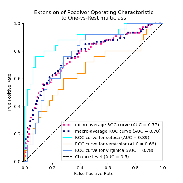
绘制所有 OvR ROC 曲线#
from itertools import cycle

fig, ax = plt.subplots(figsize=(6, 6))

plt.plot(
    fpr["micro"],
    tpr["micro"],
    label=f"micro-average ROC curve (AUC = {roc_auc['micro']:.2f})",
    color="deeppink",
    linestyle=":",
    linewidth=4,
)

plt.plot(
    fpr["macro"],
    tpr["macro"],
    label=f"macro-average ROC curve (AUC = {roc_auc['macro']:.2f})",
    color="navy",
    linestyle=":",
    linewidth=4,
)

colors = cycle(["aqua", "darkorange", "cornflowerblue"])
for class_id, color in zip(range(n_classes), colors):
    RocCurveDisplay.from_predictions(
        y_onehot_test[:, class_id],
        y_score[:, class_id],
        name=f"ROC curve for {target_names[class_id]}",
        curve_kwargs=dict(color=color),
        ax=ax,
        plot_chance_level=(class_id == 2),
        despine=True,
    )

_ = ax.set(
    xlabel="False Positive Rate",
    ylabel="True Positive Rate",
    title="Extension of Receiver Operating Characteristic\nto One-vs-Rest multiclass",
)
一对一 (One-vs-One) 多类别 ROC#
“一对一”(OvO) 多类别策略包括为每个类别对拟合一个分类器。由于它需要训练 n_classes * (n_classes - 1) / 2 个分类器,因此该方法通常比“一对多”慢,因为它具有 O(n_classes ^2) 的复杂性。
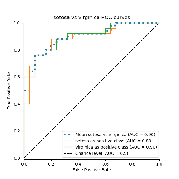
在本节中,我们演示了在 鸢尾花数据集 中,使用 OvO 方案对 3 种可能组合(“山鸢尾”vs“变色鸢尾”、“变色鸢尾”vs“维吉尼亚鸢尾”和“维吉尼亚鸢尾”vs“山鸢尾”)的宏观平均 AUC。请注意,OvO 方案未定义微观平均。
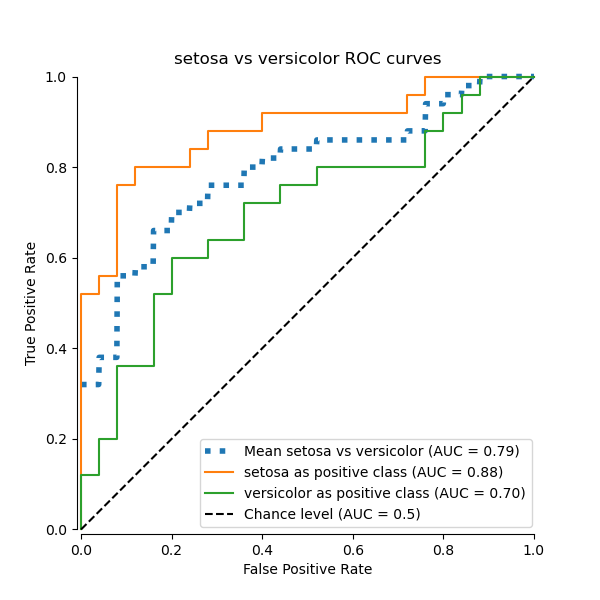
使用 OvO 宏观平均的 ROC 曲线#
在 OvO 方案中,第一步是识别所有可能的唯一对组合。分数计算通过将给定对中的一个元素视为正类别,另一个元素视为负类别来完成,然后通过反转角色并取两个分数的平均值来重新计算分数。
from itertools import combinations

pair_list = list(combinations(np.unique(y), 2))
print(pair_list)
[(np.str_('setosa'), np.str_('versicolor')), (np.str_('setosa'), np.str_('virginica')), (np.str_('versicolor'), np.str_('virginica'))]
pair_scores = []
mean_tpr = dict()

for ix, (label_a, label_b) in enumerate(pair_list):
    a_mask = y_test == label_a
    b_mask = y_test == label_b
    ab_mask = np.logical_or(a_mask, b_mask)

    a_true = a_mask[ab_mask]
    b_true = b_mask[ab_mask]

    idx_a = np.flatnonzero(label_binarizer.classes_ == label_a)[0]
    idx_b = np.flatnonzero(label_binarizer.classes_ == label_b)[0]

    fpr_a, tpr_a, _ = roc_curve(a_true, y_score[ab_mask, idx_a])
    fpr_b, tpr_b, _ = roc_curve(b_true, y_score[ab_mask, idx_b])

    mean_tpr[ix] = np.zeros_like(fpr_grid)
    mean_tpr[ix] += np.interp(fpr_grid, fpr_a, tpr_a)
    mean_tpr[ix] += np.interp(fpr_grid, fpr_b, tpr_b)
    mean_tpr[ix] /= 2
    mean_score = auc(fpr_grid, mean_tpr[ix])
    pair_scores.append(mean_score)

    fig, ax = plt.subplots(figsize=(6, 6))
    plt.plot(
        fpr_grid,
        mean_tpr[ix],
        label=f"Mean {label_a} vs {label_b} (AUC = {mean_score:.2f})",
        linestyle=":",
        linewidth=4,
    )
    RocCurveDisplay.from_predictions(
        a_true,
        y_score[ab_mask, idx_a],
        ax=ax,
        name=f"{label_a} as positive class",
    )
    RocCurveDisplay.from_predictions(
        b_true,
        y_score[ab_mask, idx_b],
        ax=ax,
        name=f"{label_b} as positive class",
        plot_chance_level=True,
        despine=True,
    )
    ax.set(
        xlabel="False Positive Rate",
        ylabel="True Positive Rate",
        title=f"{target_names[idx_a]} vs {label_b} ROC curves",
    )

print(f"Macro-averaged One-vs-One ROC AUC score:\n{np.average(pair_scores):.2f}")
Macro-averaged One-vs-One ROC AUC score:
0.78
还可以断言,我们“手动”计算的宏观平均值等同于 roc_auc_score 函数中实现的 average="macro" 选项。
macro_roc_auc_ovo = roc_auc_score(
    y_test,
    y_score,
    multi_class="ovo",
    average="macro",
)

print(f"Macro-averaged One-vs-One ROC AUC score:\n{macro_roc_auc_ovo:.2f}")
Macro-averaged One-vs-One ROC AUC score:
0.78
绘制所有 OvO ROC 曲线#
ovo_tpr = np.zeros_like(fpr_grid)

fig, ax = plt.subplots(figsize=(6, 6))
for ix, (label_a, label_b) in enumerate(pair_list):
    ovo_tpr += mean_tpr[ix]
    ax.plot(
        fpr_grid,
        mean_tpr[ix],
        label=f"Mean {label_a} vs {label_b} (AUC = {pair_scores[ix]:.2f})",
    )

ovo_tpr /= sum(1 for pair in enumerate(pair_list))

ax.plot(
    fpr_grid,
    ovo_tpr,
    label=f"One-vs-One macro-average (AUC = {macro_roc_auc_ovo:.2f})",
    linestyle=":",
    linewidth=4,
)
ax.plot([0, 1], [0, 1], "k--", label="Chance level (AUC = 0.5)")
_ = ax.set(
    xlabel="False Positive Rate",
    ylabel="True Positive Rate",
    title="Extension of Receiver Operating Characteristic\nto One-vs-One multiclass",
    aspect="equal",
    xlim=(-0.01, 1.01),
    ylim=(-0.01, 1.01),
)
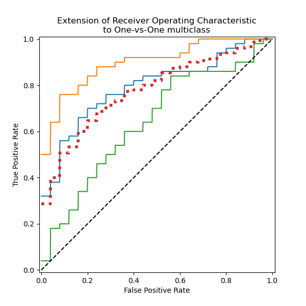
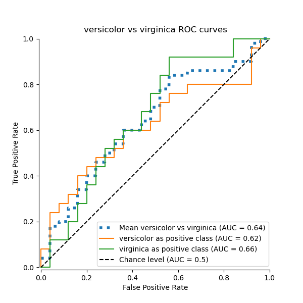
我们确认“变色鸢尾”和“维吉尼亚鸢尾”类别无法通过线性分类器很好地识别。“维吉尼亚鸢尾”vs“其余”的 ROC-AUC 分数 (0.77) 介于“变色鸢尾”vs“维吉尼亚鸢尾” (0.64) 和“山鸢尾”vs“维吉尼亚鸢尾” (0.90) 的 OvO ROC-AUC 分数之间。事实上,OvO 策略提供了关于一对类别之间混淆的额外信息,尽管当类别数量大时会增加计算成本。
如果用户主要对正确识别特定类别或类别子集感兴趣,则推荐使用 OvO 策略,而分类器的整体性能仍可通过给定的平均策略进行总结。
在处理不平衡数据集时,根据业务背景或您正在解决的问题选择适当的指标至关重要。根据期望的结果选择适当的平均方法(微观平均与宏观平均)也同样重要
微观平均聚合所有实例的指标,平等对待每个独立实例,无论其类别如何。这种方法在评估整体性能时很有用,但请注意,在不平衡数据集中,它可能被多数类别主导。
宏观平均独立计算每个类别的指标,然后取其平均值,为每个类别赋予相同的权重。当您希望将代表性不足的类别视为与高密度类别同样重要时,这尤其有用。
脚本总运行时间: (0 分 0.599 秒)
相关示例