在scikit-learn中可视化交叉验证行为#

选择正确的交叉验证对象是正确拟合模型的关键部分。有许多方法可以将数据分割为训练集和测试集，以避免模型过拟合，标准化测试集中的组数量等。

此示例可视化了几种常见 scikit-learn 对象的行为以供比较。

# Authors: The scikit-learn developers
# SPDX-License-Identifier: BSD-3-Clause

import matplotlib.pyplot as plt
import numpy as np
from matplotlib.patches import Patch

from sklearn.model_selection import (
    GroupKFold,
    GroupShuffleSplit,
    KFold,
    ShuffleSplit,
    StratifiedGroupKFold,
    StratifiedKFold,
    StratifiedShuffleSplit,
    TimeSeriesSplit,
)

rng = np.random.RandomState(1338)
cmap_data = plt.cm.Paired
cmap_cv = plt.cm.coolwarm
n_splits = 4

可视化我们的数据#

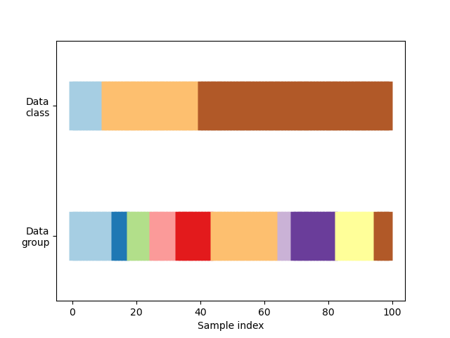
首先，我们必须理解数据的结构。它包含 100 个随机生成的输入数据点，3 个类在数据点中不均匀分布，以及 10 个“组”在数据点中均匀分布。

正如我们将看到的，一些交叉验证对象对带标签的数据执行特定操作，另一些对分组数据表现不同，还有一些不使用此信息。

首先，我们将可视化我们的数据。

# Generate the class/group data
n_points = 100
X = rng.randn(100, 10)

percentiles_classes = [0.1, 0.3, 0.6]
y = np.hstack([[ii] * int(100 * perc) for ii, perc in enumerate(percentiles_classes)])

# Generate uneven groups
group_prior = rng.dirichlet([2] * 10)
groups = np.repeat(np.arange(10), rng.multinomial(100, group_prior))


def visualize_groups(classes, groups, name):
    # Visualize dataset groups
    fig, ax = plt.subplots()
    ax.scatter(
        range(len(groups)),
        [0.5] * len(groups),
        c=groups,
        marker="_",
        lw=50,
        cmap=cmap_data,
    )
    ax.scatter(
        range(len(groups)),
        [3.5] * len(groups),
        c=classes,
        marker="_",
        lw=50,
        cmap=cmap_data,
    )
    ax.set(
        ylim=[-1, 5],
        yticks=[0.5, 3.5],
        yticklabels=["Data\ngroup", "Data\nclass"],
        xlabel="Sample index",
    )


visualize_groups(y, groups, "no groups")

定义一个函数来可视化交叉验证行为#

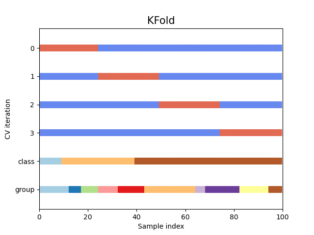
我们将定义一个函数，使我们能够可视化每个交叉验证对象的行为。我们将对数据执行 4 次分割。在每次分割中，我们将可视化为训练集（蓝色）和测试集（红色）选择的索引。

def plot_cv_indices(cv, X, y, group, ax, n_splits, lw=10):
    """Create a sample plot for indices of a cross-validation object."""
    use_groups = "Group" in type(cv).__name__
    groups = group if use_groups else None
    # Generate the training/testing visualizations for each CV split
    for ii, (tr, tt) in enumerate(cv.split(X=X, y=y, groups=groups)):
        # Fill in indices with the training/test groups
        indices = np.array([np.nan] * len(X))
        indices[tt] = 1
        indices[tr] = 0

        # Visualize the results
        ax.scatter(
            range(len(indices)),
            [ii + 0.5] * len(indices),
            c=indices,
            marker="_",
            lw=lw,
            cmap=cmap_cv,
            vmin=-0.2,
            vmax=1.2,
        )

    # Plot the data classes and groups at the end
    ax.scatter(
        range(len(X)), [ii + 1.5] * len(X), c=y, marker="_", lw=lw, cmap=cmap_data
    )

    ax.scatter(
        range(len(X)), [ii + 2.5] * len(X), c=group, marker="_", lw=lw, cmap=cmap_data
    )

    # Formatting
    yticklabels = list(range(n_splits)) + ["class", "group"]
    ax.set(
        yticks=np.arange(n_splits + 2) + 0.5,
        yticklabels=yticklabels,
        xlabel="Sample index",
        ylabel="CV iteration",
        ylim=[n_splits + 2.2, -0.2],
        xlim=[0, 100],
    )
    ax.set_title("{}".format(type(cv).__name__), fontsize=15)
    return ax

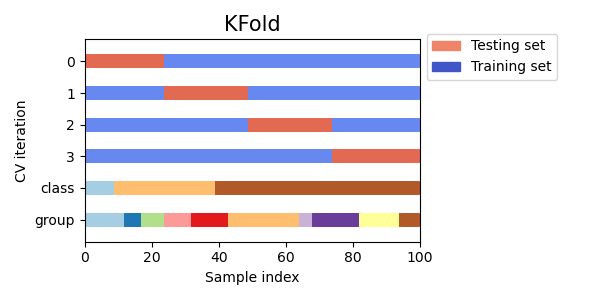
让我们看看 KFold 交叉验证对象的表现如何

fig, ax = plt.subplots()
cv = KFold(n_splits)
plot_cv_indices(cv, X, y, groups, ax, n_splits)

<Axes: title={'center': 'KFold'}, xlabel='Sample index', ylabel='CV iteration'>

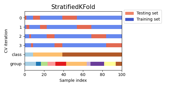
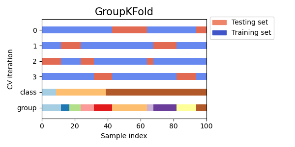
如您所见，默认情况下，KFold 交叉验证迭代器不考虑数据点类别或组。我们可以通过使用以下方法更改这一点：

使用StratifiedKFold 来保留每个类别的样本百分比。
使用GroupKFold 来确保相同的组不会出现在两个不同的折叠中。
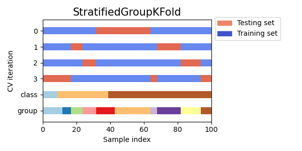
使用StratifiedGroupKFold 来保持 GroupKFold 的约束，同时尝试返回分层折叠。

cvs = [StratifiedKFold, GroupKFold, StratifiedGroupKFold]

for cv in cvs:
    fig, ax = plt.subplots(figsize=(6, 3))
    plot_cv_indices(cv(n_splits), X, y, groups, ax, n_splits)
    ax.legend(
        [Patch(color=cmap_cv(0.8)), Patch(color=cmap_cv(0.02))],
        ["Testing set", "Training set"],
        loc=(1.02, 0.8),
    )
    # Make the legend fit
    plt.tight_layout()
    fig.subplots_adjust(right=0.7)

接下来，我们将可视化多个交叉验证迭代器的这种行为。

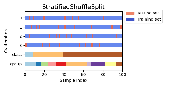
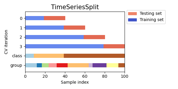
可视化多个交叉验证对象的交叉验证索引#

让我们直观地比较多个 scikit-learn 交叉验证对象的交叉验证行为。下面我们将遍历几个常见的交叉验证对象，并可视化每个对象的行为。

请注意，有些使用了组/类别信息，而另一些则没有。

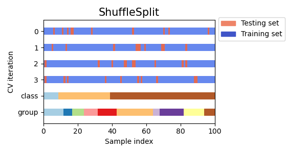
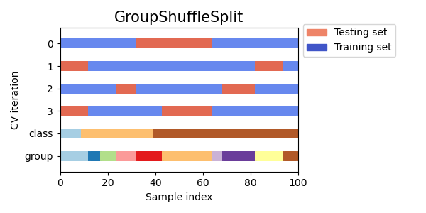
cvs = [
    KFold,
    GroupKFold,
    ShuffleSplit,
    StratifiedKFold,
    StratifiedGroupKFold,
    GroupShuffleSplit,
    StratifiedShuffleSplit,
    TimeSeriesSplit,
]


for cv in cvs:
    this_cv = cv(n_splits=n_splits)
    fig, ax = plt.subplots(figsize=(6, 3))
    plot_cv_indices(this_cv, X, y, groups, ax, n_splits)

    ax.legend(
        [Patch(color=cmap_cv(0.8)), Patch(color=cmap_cv(0.02))],
        ["Testing set", "Training set"],
        loc=(1.02, 0.8),
    )
    # Make the legend fit
    plt.tight_layout()
    fig.subplots_adjust(right=0.7)
plt.show()