最近邻分类

此示例展示了如何使用 KNeighborsClassifier。我们在鸢尾花数据集上训练这样一个分类器，并观察通过参数 weights 获得的决策边界的差异。

# Authors: The scikit-learn developers
# SPDX-License-Identifier: BSD-3-Clause

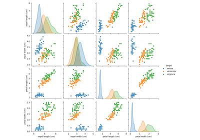
加载数据

在此示例中，我们使用鸢尾花数据集。我们将数据分为训练集和测试集。

from sklearn.datasets import load_iris
from sklearn.model_selection import train_test_split

iris = load_iris(as_frame=True)
X = iris.data[["sepal length (cm)", "sepal width (cm)"]]
y = iris.target
X_train, X_test, y_train, y_test = train_test_split(X, y, stratify=y, random_state=0)

K-最近邻分类器

我们希望使用一个 K-最近邻分类器，考虑 11 个数据点的邻域。由于我们的 K-最近邻模型使用欧几里得距离来查找最近邻，因此事先对数据进行缩放非常重要。有关更多详细信息，请参阅题为 特征缩放的重要性 的示例。

因此，我们使用 Pipeline 在使用分类器之前链式添加一个缩放器。

from sklearn.neighbors import KNeighborsClassifier
from sklearn.pipeline import Pipeline
from sklearn.preprocessing import StandardScaler

clf = Pipeline(
    steps=[("scaler", StandardScaler()), ("knn", KNeighborsClassifier(n_neighbors=11))]
)

决策边界

现在，我们拟合两个分类器，使用参数 weights 的不同值。我们绘制每个分类器的决策边界以及原始数据集，以观察差异。

import matplotlib.pyplot as plt

from sklearn.inspection import DecisionBoundaryDisplay

_, axs = plt.subplots(ncols=2, figsize=(12, 5))

for ax, weights in zip(axs, ("uniform", "distance")):
    clf.set_params(knn__weights=weights).fit(X_train, y_train)
    disp = DecisionBoundaryDisplay.from_estimator(
        clf,
        X_test,
        response_method="predict",
        plot_method="pcolormesh",
        xlabel=iris.feature_names[0],
        ylabel=iris.feature_names[1],
        shading="auto",
        alpha=0.5,
        ax=ax,
    )
    scatter = disp.ax_.scatter(X.iloc[:, 0], X.iloc[:, 1], c=y, edgecolors="k")
    disp.ax_.legend(
        scatter.legend_elements()[0],
        iris.target_names,
        loc="lower left",
        title="Classes",
    )
    _ = disp.ax_.set_title(
        f"3-Class classification\n(k={clf[-1].n_neighbors}, weights={weights!r})"
    )

plt.show()

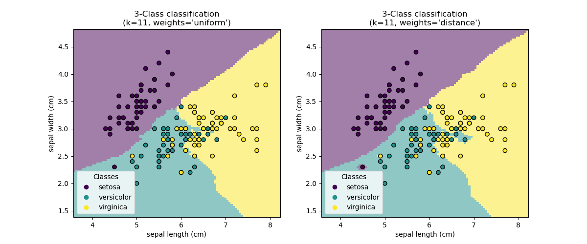
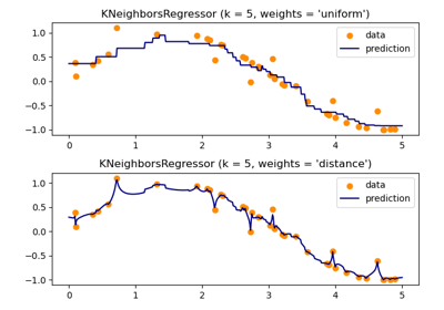
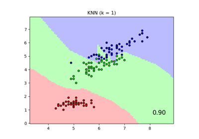
结论

我们观察到参数 weights 对决策边界有影响。当 weights="unifom" 时，所有最近邻对决策的影响相同。而当 weights="distance" 时，赋予每个邻居的权重与该邻居到查询点的距离的倒数成比例。

在某些情况下，考虑距离可能会改善模型。

相关示例

最近邻回归

最近邻回归

比较带和不带邻域成分分析的最近邻

比较带和不带邻域成分分析的最近邻

缓存最近邻

缓存最近邻

鸢尾花数据集上的主成分分析 (PCA)

鸢尾花数据集上的主成分分析 (PCA)