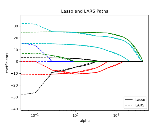
Lasso、Lasso-LARS 和弹性网络路径#

本示例展示了如何计算 Lasso、Lasso-LARS 和弹性网络正则化路径上的系数“路径”。换句话说，它显示了正则化参数（alpha）与系数之间的关系。

Lasso 和 Lasso-LARS 对系数施加了稀疏性约束，鼓励其中一些变为零。弹性网络是 Lasso 的推广，它在 L1 惩罚项的基础上增加了 L2 惩罚项。这使得一些系数可以非零，同时仍然鼓励稀疏性。

Lasso 和弹性网络使用坐标下降法计算路径，而 Lasso-LARS 使用 LARS 算法计算路径。

路径使用 lasso_path、lars_path 和 enet_path 计算。

结果显示了不同的比较图：

比较 Lasso 和 Lasso-LARS
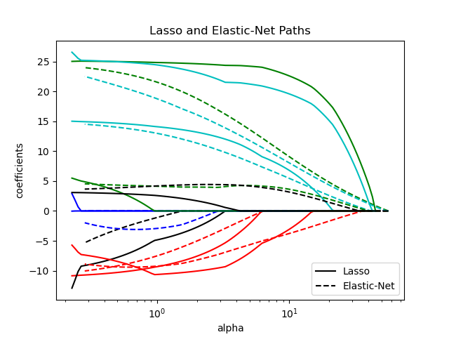
比较 Lasso 和弹性网络
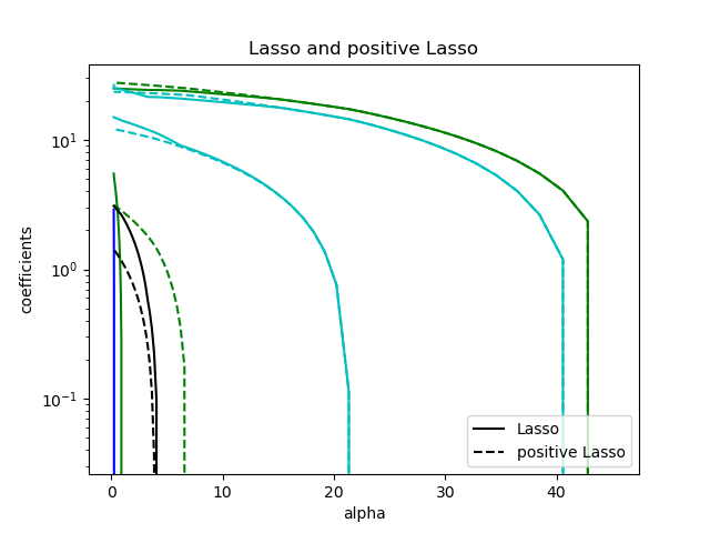
比较 Lasso 和正 Lasso
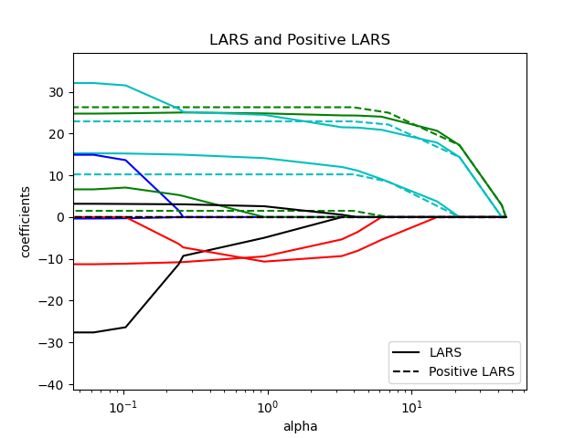
比较 LARS 和正 LARS
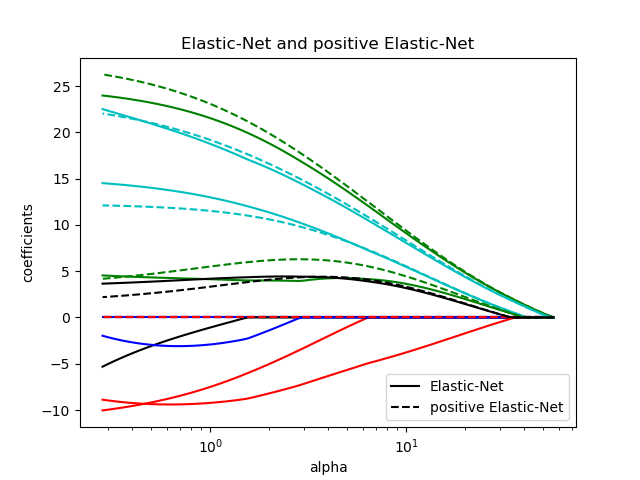
比较弹性网络和正弹性网络

每个图都显示了模型系数如何随正则化强度变化，提供了对这些模型在不同约束下行为的洞察。

Computing regularization path using the lasso...
Computing regularization path using the positive lasso...
Computing regularization path using the LARS...
Computing regularization path using the positive LARS...
Computing regularization path using the elastic net...
Computing regularization path using the positive elastic net...

# Authors: The scikit-learn developers
# SPDX-License-Identifier: BSD-3-Clause

from itertools import cycle

import matplotlib.pyplot as plt

from sklearn.datasets import load_diabetes
from sklearn.linear_model import enet_path, lars_path, lasso_path

X, y = load_diabetes(return_X_y=True)
X /= X.std(axis=0)  # Standardize data (easier to set the l1_ratio parameter)

# Compute paths

eps = 5e-3  # the smaller it is the longer is the path

print("Computing regularization path using the lasso...")
alphas_lasso, coefs_lasso, _ = lasso_path(X, y, eps=eps)

print("Computing regularization path using the positive lasso...")
alphas_positive_lasso, coefs_positive_lasso, _ = lasso_path(
    X, y, eps=eps, positive=True
)

print("Computing regularization path using the LARS...")
alphas_lars, _, coefs_lars = lars_path(X, y, method="lasso")

print("Computing regularization path using the positive LARS...")
alphas_positive_lars, _, coefs_positive_lars = lars_path(
    X, y, method="lasso", positive=True
)

print("Computing regularization path using the elastic net...")
alphas_enet, coefs_enet, _ = enet_path(X, y, eps=eps, l1_ratio=0.8)

print("Computing regularization path using the positive elastic net...")
alphas_positive_enet, coefs_positive_enet, _ = enet_path(
    X, y, eps=eps, l1_ratio=0.8, positive=True
)

# Display results

plt.figure(1)
colors = cycle(["b", "r", "g", "c", "k"])
for coef_lasso, coef_lars, c in zip(coefs_lasso, coefs_lars, colors):
    l1 = plt.semilogx(alphas_lasso, coef_lasso, c=c)
    l2 = plt.semilogx(alphas_lars, coef_lars, linestyle="--", c=c)

plt.xlabel("alpha")
plt.ylabel("coefficients")
plt.title("Lasso and LARS Paths")
plt.legend((l1[-1], l2[-1]), ("Lasso", "LARS"), loc="lower right")
plt.axis("tight")

plt.figure(2)
colors = cycle(["b", "r", "g", "c", "k"])
for coef_l, coef_e, c in zip(coefs_lasso, coefs_enet, colors):
    l1 = plt.semilogx(alphas_lasso, coef_l, c=c)
    l2 = plt.semilogx(alphas_enet, coef_e, linestyle="--", c=c)

plt.xlabel("alpha")
plt.ylabel("coefficients")
plt.title("Lasso and Elastic-Net Paths")
plt.legend((l1[-1], l2[-1]), ("Lasso", "Elastic-Net"), loc="lower right")
plt.axis("tight")


plt.figure(3)
for coef_l, coef_pl, c in zip(coefs_lasso, coefs_positive_lasso, colors):
    l1 = plt.semilogy(alphas_lasso, coef_l, c=c)
    l2 = plt.semilogy(alphas_positive_lasso, coef_pl, linestyle="--", c=c)

plt.xlabel("alpha")
plt.ylabel("coefficients")
plt.title("Lasso and positive Lasso")
plt.legend((l1[-1], l2[-1]), ("Lasso", "positive Lasso"), loc="lower right")
plt.axis("tight")


plt.figure(4)
colors = cycle(["b", "r", "g", "c", "k"])
for coef_lars, coef_positive_lars, c in zip(coefs_lars, coefs_positive_lars, colors):
    l1 = plt.semilogx(alphas_lars, coef_lars, c=c)
    l2 = plt.semilogx(alphas_positive_lars, coef_positive_lars, linestyle="--", c=c)

plt.xlabel("alpha")
plt.ylabel("coefficients")
plt.title("LARS and Positive LARS")
plt.legend((l1[-1], l2[-1]), ("LARS", "Positive LARS"), loc="lower right")
plt.axis("tight")

plt.figure(5)
for coef_e, coef_pe, c in zip(coefs_enet, coefs_positive_enet, colors):
    l1 = plt.semilogx(alphas_enet, coef_e, c=c)
    l2 = plt.semilogx(alphas_positive_enet, coef_pe, linestyle="--", c=c)

plt.xlabel("alpha")
plt.ylabel("coefficients")
plt.title("Elastic-Net and positive Elastic-Net")
plt.legend((l1[-1], l2[-1]), ("Elastic-Net", "positive Elastic-Net"), loc="lower right")
plt.axis("tight")
plt.show()

脚本总运行时间： (0 分 0.886 秒)

Lasso、Lasso-LARS 和弹性网络路径#

本页