机器学习无法推断因果效应#

机器学习模型非常擅长衡量统计关联。不幸的是，除非我们愿意对数据做出强假设，否则这些模型无法推断因果效应。

为了说明这一点，我们将模拟一个场景，尝试回答教育经济学中最重要的问题之一：获得大学学位对每小时工资的因果效应是什么？ 尽管这个问题的答案对政策制定者至关重要，但遗漏变量偏差 (OVB) 阻碍了我们识别这种因果效应。

# Authors: The scikit-learn developers
# SPDX-License-Identifier: BSD-3-Clause

数据集：模拟每小时工资#

数据生成过程在下面的代码中列出。工龄和能力衡量指标取自正态分布；父母一方的每小时工资取自 Beta 分布。然后，我们创建一个大学学位指标，该指标受到能力和父母每小时工资的积极影响。最后，我们将每小时工资建模为所有先前变量的线性函数和一个随机分量。请注意，所有变量都对每小时工资有积极影响。

import numpy as np
import pandas as pd

n_samples = 10_000
rng = np.random.RandomState(32)

experiences = rng.normal(20, 10, size=n_samples).astype(int)
experiences[experiences < 0] = 0
abilities = rng.normal(0, 0.15, size=n_samples)
parent_hourly_wages = 50 * rng.beta(2, 8, size=n_samples)
parent_hourly_wages[parent_hourly_wages < 0] = 0
college_degrees = (
    9 * abilities + 0.02 * parent_hourly_wages + rng.randn(n_samples) > 0.7
).astype(int)

true_coef = pd.Series(
    {
        "college degree": 2.0,
        "ability": 5.0,
        "experience": 0.2,
        "parent hourly wage": 1.0,
    }
)
hourly_wages = (
    true_coef["experience"] * experiences
    + true_coef["parent hourly wage"] * parent_hourly_wages
    + true_coef["college degree"] * college_degrees
    + true_coef["ability"] * abilities
    + rng.normal(0, 1, size=n_samples)
)

hourly_wages[hourly_wages < 0] = 0

模拟数据描述#

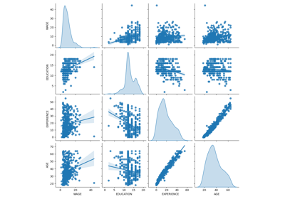
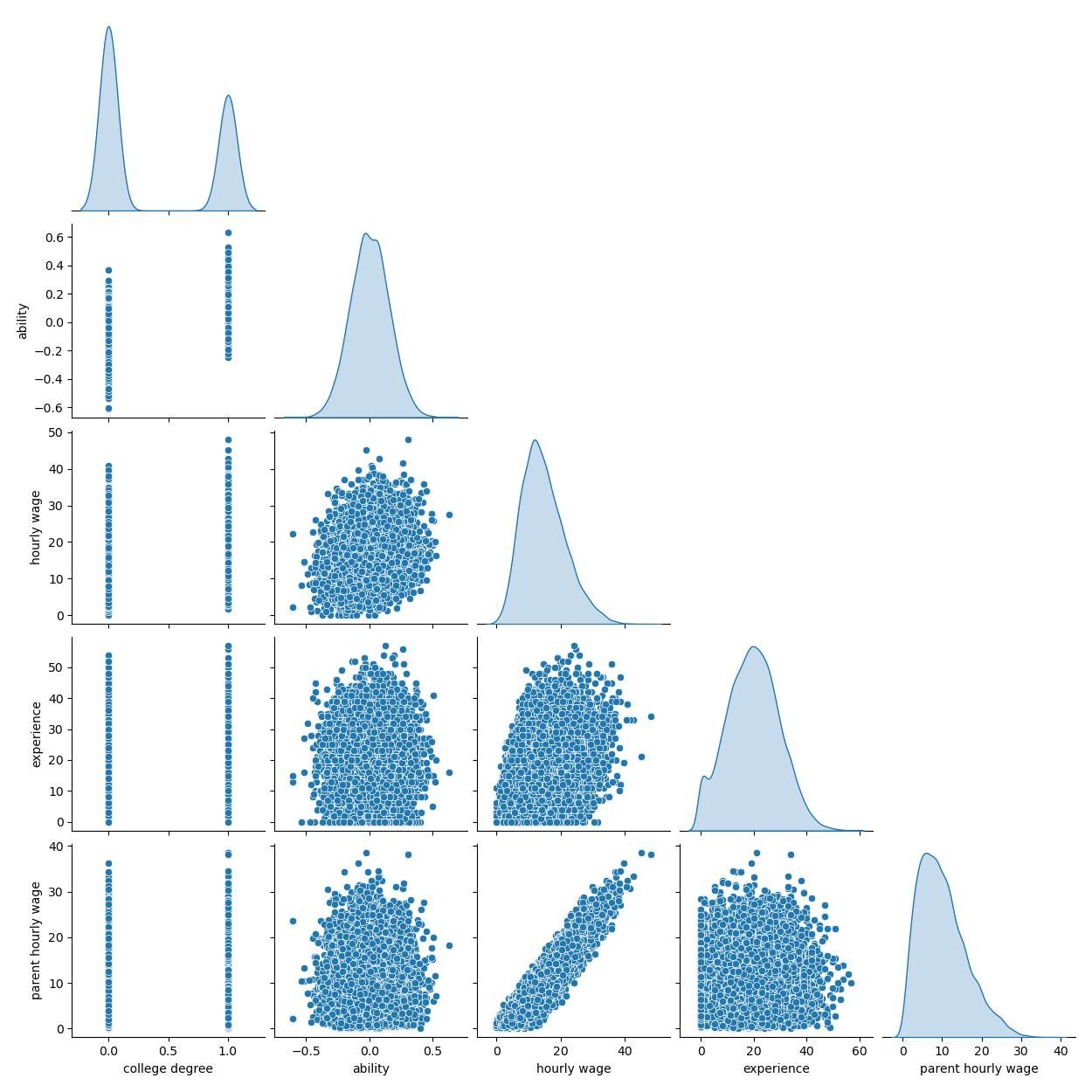
下图显示了每个变量的分布以及成对散点图。我们 OVB 故事的关键是能力和大学学位之间的正相关关系。

import seaborn as sns

df = pd.DataFrame(
    {
        "college degree": college_degrees,
        "ability": abilities,
        "hourly wage": hourly_wages,
        "experience": experiences,
        "parent hourly wage": parent_hourly_wages,
    }
)

grid = sns.pairplot(df, diag_kind="kde", corner=True)

在下一节中，我们将训练预测模型，因此我们将目标列与特征分开，并将数据拆分为训练集和测试集。

from sklearn.model_selection import train_test_split

target_name = "hourly wage"
X, y = df.drop(columns=target_name), df[target_name]
X_train, X_test, y_train, y_test = train_test_split(X, y, test_size=0.2, random_state=0)

使用完全观测变量的收入预测#

首先，我们训练一个预测模型，一个 LinearRegression 模型。在此实验中，我们假设真实生成模型使用的所有变量都可用。

from sklearn.linear_model import LinearRegression
from sklearn.metrics import r2_score

features_names = ["experience", "parent hourly wage", "college degree", "ability"]

regressor_with_ability = LinearRegression()
regressor_with_ability.fit(X_train[features_names], y_train)
y_pred_with_ability = regressor_with_ability.predict(X_test[features_names])
R2_with_ability = r2_score(y_test, y_pred_with_ability)

print(f"R2 score with ability: {R2_with_ability:.3f}")

R2 score with ability: 0.975

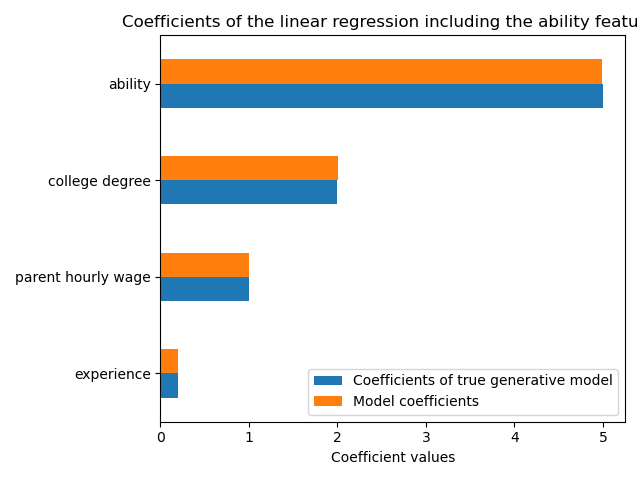
该模型能很好地预测每小时工资，R2 分数很高。我们绘制模型系数以显示我们精确地恢复了真实生成模型的值。

import matplotlib.pyplot as plt

model_coef = pd.Series(regressor_with_ability.coef_, index=features_names)
coef = pd.concat(
    [true_coef[features_names], model_coef],
    keys=["Coefficients of true generative model", "Model coefficients"],
    axis=1,
)
ax = coef.plot.barh()
ax.set_xlabel("Coefficient values")
ax.set_title("Coefficients of the linear regression including the ability features")
_ = plt.tight_layout()

Coefficients of the linear regression including the ability features

使用部分观测的收入预测#

在实践中，智力能力通常无法观测，或者只能通过无意中也衡量教育的替代指标（例如 IQ 测试）来估计。但是，从线性模型中省略“能力”特征会通过正向 OVB 夸大估计值。

features_names = ["experience", "parent hourly wage", "college degree"]

regressor_without_ability = LinearRegression()
regressor_without_ability.fit(X_train[features_names], y_train)
y_pred_without_ability = regressor_without_ability.predict(X_test[features_names])
R2_without_ability = r2_score(y_test, y_pred_without_ability)

print(f"R2 score without ability: {R2_without_ability:.3f}")

R2 score without ability: 0.968

当我们省略能力特征时，模型的预测能力在 R2 分数方面相似。我们现在检查模型的系数是否与真实生成模型不同。

model_coef = pd.Series(regressor_without_ability.coef_, index=features_names)
coef = pd.concat(
    [true_coef[features_names], model_coef],
    keys=["Coefficients of true generative model", "Model coefficients"],
    axis=1,
)
ax = coef.plot.barh()
ax.set_xlabel("Coefficient values")
_ = ax.set_title("Coefficients of the linear regression excluding the ability feature")
plt.tight_layout()
plt.show()

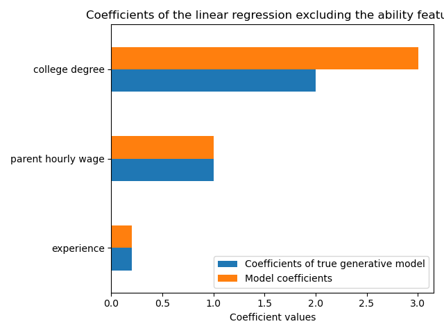
Coefficients of the linear regression excluding the ability feature

为了弥补遗漏变量，模型夸大了大学学位特征的系数。因此，将此系数值解释为真实生成模型的因果效应是错误的。

经验教训#

机器学习模型并非设计用于估计因果效应。虽然我们用线性模型展示了这一点，但 OVB 会影响任何类型的模型。

在解释系数或由特征变化引起的预测变化时，重要的是要记住可能存在与相关特征和目标变量都相关的未观测变量。这些变量被称为混淆变量。为了在存在混淆的情况下仍能估计因果效应，研究人员通常会进行实验，其中处理变量（例如大学学位）是随机化的。当实验成本过高或不道德时，研究人员有时可以使用其他因果推断技术，例如工具变量 (IV) 估计。

脚本总运行时间： (0 分钟 2.088 秒)