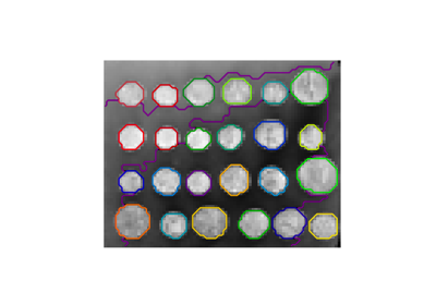
将希腊硬币图片分割成区域#

本示例使用谱聚类对图像上由体素间差异生成的图进行处理，以将该图像分割成多个部分同质区域。

此过程（图像上的谱聚类）是寻找归一化图割的有效近似解。

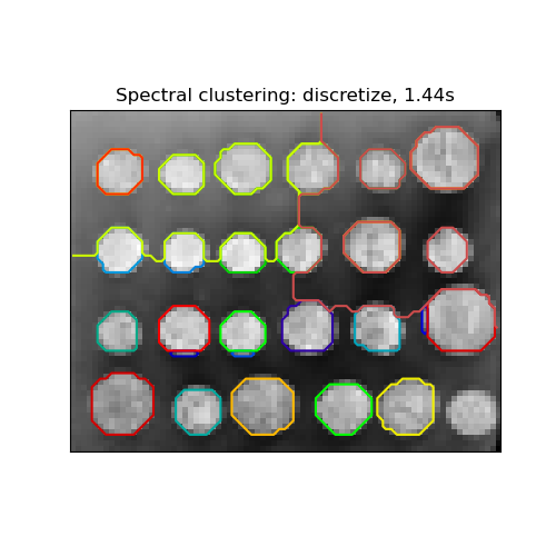
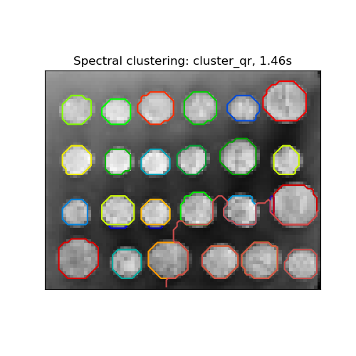
有三种分配标签的选项

“kmeans”谱聚类使用 K-Means 算法在嵌入空间中对样本进行聚类。
“discrete”迭代搜索最接近谱聚类嵌入空间的划分空间。
“cluster_qr”使用带主元分解的 QR 分解来分配标签，这直接决定了嵌入空间中的划分。

# Authors: The scikit-learn developers
# SPDX-License-Identifier: BSD-3-Clause

import time

import matplotlib.pyplot as plt
import numpy as np
from scipy.ndimage import gaussian_filter
from skimage.data import coins
from skimage.transform import rescale

from sklearn.cluster import spectral_clustering
from sklearn.feature_extraction import image

# load the coins as a numpy array
orig_coins = coins()

# Resize it to 20% of the original size to speed up the processing
# Applying a Gaussian filter for smoothing prior to down-scaling
# reduces aliasing artifacts.
smoothened_coins = gaussian_filter(orig_coins, sigma=2)
rescaled_coins = rescale(smoothened_coins, 0.2, mode="reflect", anti_aliasing=False)

# Convert the image into a graph with the value of the gradient on the
# edges.
graph = image.img_to_graph(rescaled_coins)

# Take a decreasing function of the gradient: an exponential
# The smaller beta is, the more independent the segmentation is of the
# actual image. For beta=1, the segmentation is close to a voronoi
beta = 10
eps = 1e-6
graph.data = np.exp(-beta * graph.data / graph.data.std()) + eps

# The number of segmented regions to display needs to be chosen manually.
# The current version of 'spectral_clustering' does not support determining
# the number of good quality clusters automatically.
n_regions = 26

计算并可视化结果区域

# Computing a few extra eigenvectors may speed up the eigen_solver.
# The spectral clustering quality may also benefit from requesting
# extra regions for segmentation.
n_regions_plus = 3

# Apply spectral clustering using the default eigen_solver='arpack'.
# Any implemented solver can be used: eigen_solver='arpack', 'lobpcg', or 'amg'.
# Choosing eigen_solver='amg' requires an extra package called 'pyamg'.
# The quality of segmentation and the speed of calculations is mostly determined
# by the choice of the solver and the value of the tolerance 'eigen_tol'.
# TODO: varying eigen_tol seems to have no effect for 'lobpcg' and 'amg' #21243.
for assign_labels in ("kmeans", "discretize", "cluster_qr"):
    t0 = time.time()
    labels = spectral_clustering(
        graph,
        n_clusters=(n_regions + n_regions_plus),
        eigen_tol=1e-7,
        assign_labels=assign_labels,
        random_state=42,
    )

    t1 = time.time()
    labels = labels.reshape(rescaled_coins.shape)
    plt.figure(figsize=(5, 5))
    plt.imshow(rescaled_coins, cmap=plt.cm.gray)

    plt.xticks(())
    plt.yticks(())
    title = "Spectral clustering: %s, %.2fs" % (assign_labels, (t1 - t0))
    print(title)
    plt.title(title)
    for l in range(n_regions):
        colors = [plt.cm.nipy_spectral((l + 4) / float(n_regions + 4))]
        plt.contour(labels == l, colors=colors)
        # To view individual segments as appear comment in plt.pause(0.5)
plt.show()

# TODO: After #21194 is merged and #21243 is fixed, check which eigen_solver
# is the best and set eigen_solver='arpack', 'lobpcg', or 'amg' and eigen_tol
# explicitly in this example.

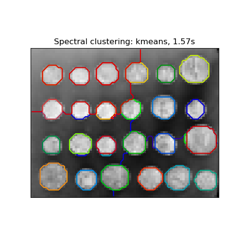
Spectral clustering: kmeans, 1.57s
Spectral clustering: discretize, 1.44s
Spectral clustering: cluster_qr, 1.46s

脚本总运行时间： (0 分 4.828 秒)

将希腊硬币图片分割成区域#

本页