梯度提升中的类别特征支持#

在此示例中，我们将比较HistGradientBoostingRegressor在不同类别特征编码策略下的训练时间和预测性能。具体来说，我们将评估

丢弃类别特征
使用OneHotEncoder
使用OrdinalEncoder并将类别视为有序、等距的量
使用OrdinalEncoder并依赖HistGradientBoostingRegressor估计器的原生类别支持。

我们将使用Ames爱荷华州住房数据集，该数据集包含数值和类别特征，其中房屋的销售价格是目标。

有关展示HistGradientBoostingRegressor其他一些特征的示例，请参阅直方图梯度提升树中的特征。

# Authors: The scikit-learn developers
# SPDX-License-Identifier: BSD-3-Clause

加载Ames住房数据集#

首先，我们将Ames住房数据加载为pandas数据帧。特征可以是类别型或数值型。

from sklearn.datasets import fetch_openml

X, y = fetch_openml(data_id=42165, as_frame=True, return_X_y=True)

# Select only a subset of features of X to make the example faster to run
categorical_columns_subset = [
    "BldgType",
    "GarageFinish",
    "LotConfig",
    "Functional",
    "MasVnrType",
    "HouseStyle",
    "FireplaceQu",
    "ExterCond",
    "ExterQual",
    "PoolQC",
]

numerical_columns_subset = [
    "3SsnPorch",
    "Fireplaces",
    "BsmtHalfBath",
    "HalfBath",
    "GarageCars",
    "TotRmsAbvGrd",
    "BsmtFinSF1",
    "BsmtFinSF2",
    "GrLivArea",
    "ScreenPorch",
]

X = X[categorical_columns_subset + numerical_columns_subset]
X[categorical_columns_subset] = X[categorical_columns_subset].astype("category")

categorical_columns = X.select_dtypes(include="category").columns
n_categorical_features = len(categorical_columns)
n_numerical_features = X.select_dtypes(include="number").shape[1]

print(f"Number of samples: {X.shape[0]}")
print(f"Number of features: {X.shape[1]}")
print(f"Number of categorical features: {n_categorical_features}")
print(f"Number of numerical features: {n_numerical_features}")

Number of samples: 1460
Number of features: 20
Number of categorical features: 10
Number of numerical features: 10

丢弃类别特征的梯度提升估计器#

作为基线，我们创建一个丢弃类别特征的估计器。

from sklearn.compose import make_column_selector, make_column_transformer
from sklearn.ensemble import HistGradientBoostingRegressor
from sklearn.pipeline import make_pipeline

dropper = make_column_transformer(
    ("drop", make_column_selector(dtype_include="category")), remainder="passthrough"
)
hist_dropped = make_pipeline(dropper, HistGradientBoostingRegressor(random_state=42))

独热编码的梯度提升估计器#

接下来，我们创建一个流水线，它将对类别特征进行独热编码，并让其余数值数据直接通过。

from sklearn.preprocessing import OneHotEncoder

one_hot_encoder = make_column_transformer(
    (
        OneHotEncoder(sparse_output=False, handle_unknown="ignore"),
        make_column_selector(dtype_include="category"),
    ),
    remainder="passthrough",
)

hist_one_hot = make_pipeline(
    one_hot_encoder, HistGradientBoostingRegressor(random_state=42)
)

有序编码的梯度提升估计器#

接下来，我们创建一个流水线，它将类别特征视为有序量，即类别将被编码为0、1、2等，并被视为连续特征。

import numpy as np

from sklearn.preprocessing import OrdinalEncoder

ordinal_encoder = make_column_transformer(
    (
        OrdinalEncoder(handle_unknown="use_encoded_value", unknown_value=np.nan),
        make_column_selector(dtype_include="category"),
    ),
    remainder="passthrough",
    # Use short feature names to make it easier to specify the categorical
    # variables in the HistGradientBoostingRegressor in the next step
    # of the pipeline.
    verbose_feature_names_out=False,
)

hist_ordinal = make_pipeline(
    ordinal_encoder, HistGradientBoostingRegressor(random_state=42)
)

支持原生类别的梯度提升估计器#

现在我们创建一个HistGradientBoostingRegressor估计器，它将原生处理类别特征。此估计器不会将类别特征视为有序量。我们设置categorical_features="from_dtype"，以便具有类别dtype的特征被视为类别特征。

此估计器与前一个估计器之间的主要区别在于，在此估计器中，我们让HistGradientBoostingRegressor从DataFrame列的dtype中检测哪些特征是类别特征。

hist_native = HistGradientBoostingRegressor(
    random_state=42, categorical_features="from_dtype"
)

模型比较#

最后，我们使用交叉验证评估模型。这里我们比较模型在平均绝对百分比误差和拟合时间方面的性能。

import matplotlib.pyplot as plt

from sklearn.model_selection import cross_validate

scoring = "neg_mean_absolute_percentage_error"
n_cv_folds = 3

dropped_result = cross_validate(hist_dropped, X, y, cv=n_cv_folds, scoring=scoring)
one_hot_result = cross_validate(hist_one_hot, X, y, cv=n_cv_folds, scoring=scoring)
ordinal_result = cross_validate(hist_ordinal, X, y, cv=n_cv_folds, scoring=scoring)
native_result = cross_validate(hist_native, X, y, cv=n_cv_folds, scoring=scoring)


def plot_results(figure_title):
    fig, (ax1, ax2) = plt.subplots(1, 2, figsize=(12, 8))

    plot_info = [
        ("fit_time", "Fit times (s)", ax1, None),
        ("test_score", "Mean Absolute Percentage Error", ax2, None),
    ]

    x, width = np.arange(4), 0.9
    for key, title, ax, y_limit in plot_info:
        items = [
            dropped_result[key],
            one_hot_result[key],
            ordinal_result[key],
            native_result[key],
        ]

        mape_cv_mean = [np.mean(np.abs(item)) for item in items]
        mape_cv_std = [np.std(item) for item in items]

        ax.bar(
            x=x,
            height=mape_cv_mean,
            width=width,
            yerr=mape_cv_std,
            color=["C0", "C1", "C2", "C3"],
        )
        ax.set(
            xlabel="Model",
            title=title,
            xticks=x,
            xticklabels=["Dropped", "One Hot", "Ordinal", "Native"],
            ylim=y_limit,
        )
    fig.suptitle(figure_title)


plot_results("Gradient Boosting on Ames Housing")

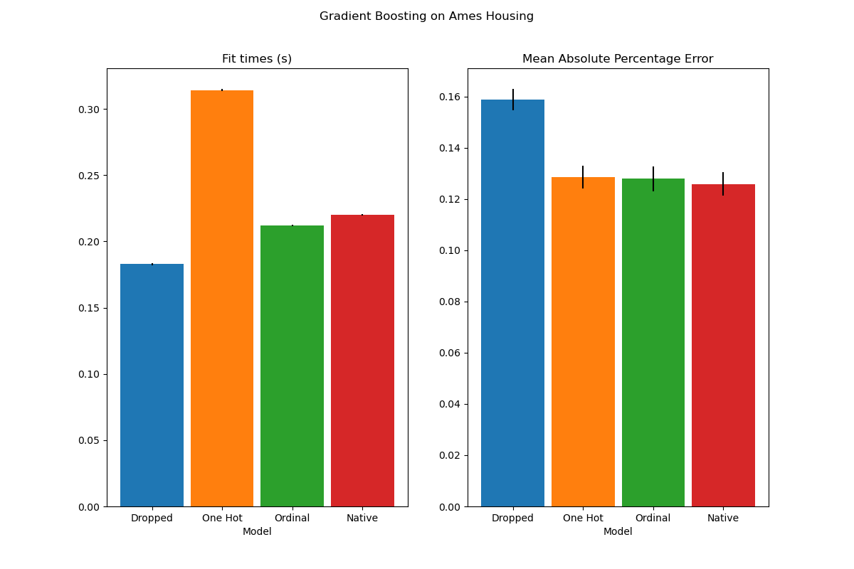
Gradient Boosting on Ames Housing, Fit times (s), Mean Absolute Percentage Error

我们看到独热编码数据的模型是迄今为止最慢的。这是意料之中的，因为独热编码为每个类别值（对于每个类别特征）创建一个额外的特征，因此在拟合过程中需要考虑更多的分裂点。理论上，我们预计类别特征的原生处理会比将类别视为有序量（“有序”）略慢，因为原生处理需要排序类别。然而，当类别数量较少时，拟合时间应该接近，这在实践中可能并非总是如此。

在预测性能方面，丢弃类别特征会导致较差的性能。使用类别特征的三个模型具有可比的错误率，其中原生处理略有优势。

限制分裂次数#

通常，独热编码的数据可能会导致较差的预测，特别是当树的深度或节点数量有限时：对于独热编码的数据，需要更多的分裂点，即更深的深度，才能恢复与原生处理中通过单个分裂点获得的等效分裂。

当类别被视为有序量时，这也同样适用：如果类别是A..F，最佳分裂是ACF - BDE，那么独热编码模型将需要3个分裂点（左侧节点中每个类别一个），而有序非原生模型将需要4个分裂点：1个分裂点用于隔离A，1个分裂点用于隔离F，以及2个分裂点用于将C从BCDE中隔离出来。

模型性能在实践中差异有多大将取决于数据集和树的灵活性。

为此，我们使用欠拟合模型重新运行相同的分析，其中我们通过限制树的数量和每棵树的深度来人为地限制总分裂次数。

for pipe in (hist_dropped, hist_one_hot, hist_ordinal, hist_native):
    if pipe is hist_native:
        # The native model does not use a pipeline so, we can set the parameters
        # directly.
        pipe.set_params(max_depth=3, max_iter=15)
    else:
        pipe.set_params(
            histgradientboostingregressor__max_depth=3,
            histgradientboostingregressor__max_iter=15,
        )

dropped_result = cross_validate(hist_dropped, X, y, cv=n_cv_folds, scoring=scoring)
one_hot_result = cross_validate(hist_one_hot, X, y, cv=n_cv_folds, scoring=scoring)
ordinal_result = cross_validate(hist_ordinal, X, y, cv=n_cv_folds, scoring=scoring)
native_result = cross_validate(hist_native, X, y, cv=n_cv_folds, scoring=scoring)

plot_results("Gradient Boosting on Ames Housing (few and small trees)")

plt.show()

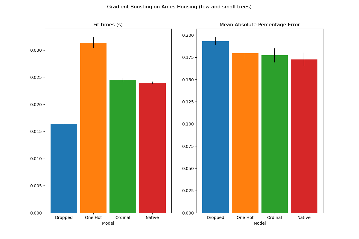
Gradient Boosting on Ames Housing (few and small trees), Fit times (s), Mean Absolute Percentage Error

这些欠拟合模型的结果证实了我们之前的直觉：当分裂预算受限时，原生类别处理策略表现最佳。另外两种策略（独热编码和将类别视为有序值）导致的错误值与完全丢弃类别特征的基线模型相当。

脚本总运行时间：(0分钟 3.595秒)