高斯过程回归：基本入门示例#

一个简单的一维回归示例，通过两种不同方式计算

无噪声情况
有噪声情况，每个数据点噪声水平已知

在这两种情况下，核函数的参数均使用最大似然原理进行估计。

这些图示了高斯过程模型的插值特性以及其概率性质（以逐点 95% 置信区间形式表示）。

请注意，alpha 是一个参数，用于控制 Tikhonov 正则化在假设的训练点协方差矩阵上的强度。

# Authors: The scikit-learn developers
# SPDX-License-Identifier: BSD-3-Clause

数据集生成#

我们将从生成一个合成数据集开始。真实的生成过程定义为 \(f(x) = x \sin(x)\)。

import numpy as np

X = np.linspace(start=0, stop=10, num=1_000).reshape(-1, 1)
y = np.squeeze(X * np.sin(X))

import matplotlib.pyplot as plt

plt.plot(X, y, label=r"$f(x) = x \sin(x)$", linestyle="dotted")
plt.legend()
plt.xlabel("$x$")
plt.ylabel("$f(x)$")
_ = plt.title("True generative process")

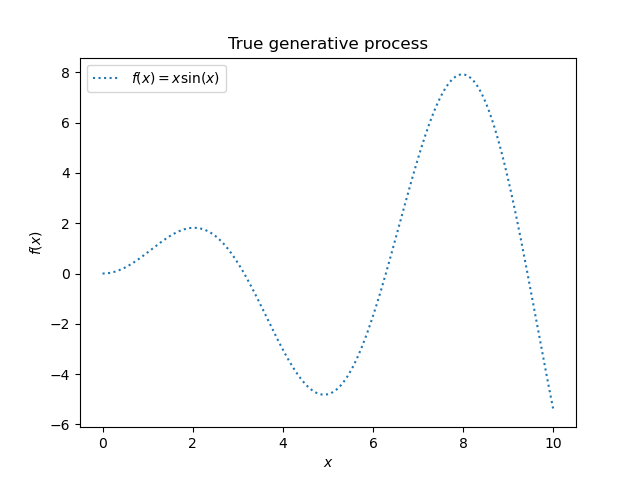
我们将在下一个实验中使用此数据集来演示高斯过程回归的工作原理。

无噪声目标示例#

在此第一个示例中，我们将使用真实的生成过程，而不添加任何噪声。为了训练高斯过程回归，我们只选择少量样本。

rng = np.random.RandomState(1)
training_indices = rng.choice(np.arange(y.size), size=6, replace=False)
X_train, y_train = X[training_indices], y[training_indices]

现在，我们对这些少量训练数据样本拟合高斯过程。我们将使用径向基函数 (RBF) 核和一个常数参数来拟合振幅。

from sklearn.gaussian_process import GaussianProcessRegressor
from sklearn.gaussian_process.kernels import RBF

kernel = 1 * RBF(length_scale=1.0, length_scale_bounds=(1e-2, 1e2))
gaussian_process = GaussianProcessRegressor(kernel=kernel, n_restarts_optimizer=9)
gaussian_process.fit(X_train, y_train)
gaussian_process.kernel_

5.02**2 * RBF(length_scale=1.43)

在拟合模型后，我们看到核函数的超参数已得到优化。现在，我们将使用我们的核函数计算完整数据集的平均预测并绘制 95% 置信区间。

mean_prediction, std_prediction = gaussian_process.predict(X, return_std=True)

plt.plot(X, y, label=r"$f(x) = x \sin(x)$", linestyle="dotted")
plt.scatter(X_train, y_train, label="Observations")
plt.plot(X, mean_prediction, label="Mean prediction")
plt.fill_between(
    X.ravel(),
    mean_prediction - 1.96 * std_prediction,
    mean_prediction + 1.96 * std_prediction,
    alpha=0.5,
    label=r"95% confidence interval",
)
plt.legend()
plt.xlabel("$x$")
plt.ylabel("$f(x)$")
_ = plt.title("Gaussian process regression on noise-free dataset")

Gaussian process regression on noise-free dataset

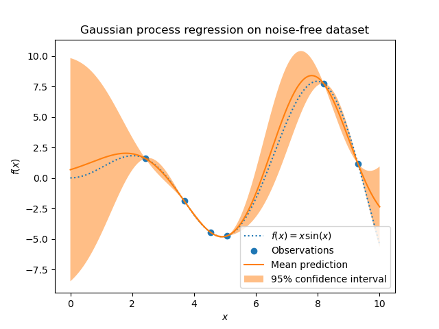
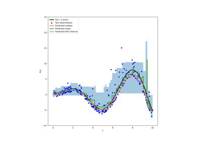
我们看到，对于在靠近训练集的数据点上进行的预测，95% 置信区间具有较小的幅度。当样本远离训练数据时，我们模型的预测准确性较低，且模型预测的精确度也较低（不确定性更高）。

有噪声目标示例#

这次我们可以重复一个类似的实验，向目标添加额外的噪声。这将允许我们看到噪声对拟合模型的影响。

我们向目标添加了一些具有任意标准差的随机高斯噪声。

noise_std = 0.75
y_train_noisy = y_train + rng.normal(loc=0.0, scale=noise_std, size=y_train.shape)

我们创建一个类似的高斯过程模型。除了核函数外，这次我们指定了参数 alpha，它可以解释为高斯噪声的方差。

gaussian_process = GaussianProcessRegressor(
    kernel=kernel, alpha=noise_std**2, n_restarts_optimizer=9
)
gaussian_process.fit(X_train, y_train_noisy)
mean_prediction, std_prediction = gaussian_process.predict(X, return_std=True)

让我们像以前一样绘制平均预测和不确定性区域。

plt.plot(X, y, label=r"$f(x) = x \sin(x)$", linestyle="dotted")
plt.errorbar(
    X_train,
    y_train_noisy,
    noise_std,
    linestyle="None",
    color="tab:blue",
    marker=".",
    markersize=10,
    label="Observations",
)
plt.plot(X, mean_prediction, label="Mean prediction")
plt.fill_between(
    X.ravel(),
    mean_prediction - 1.96 * std_prediction,
    mean_prediction + 1.96 * std_prediction,
    color="tab:orange",
    alpha=0.5,
    label=r"95% confidence interval",
)
plt.legend()
plt.xlabel("$x$")
plt.ylabel("$f(x)$")
_ = plt.title("Gaussian process regression on a noisy dataset")

Gaussian process regression on a noisy dataset

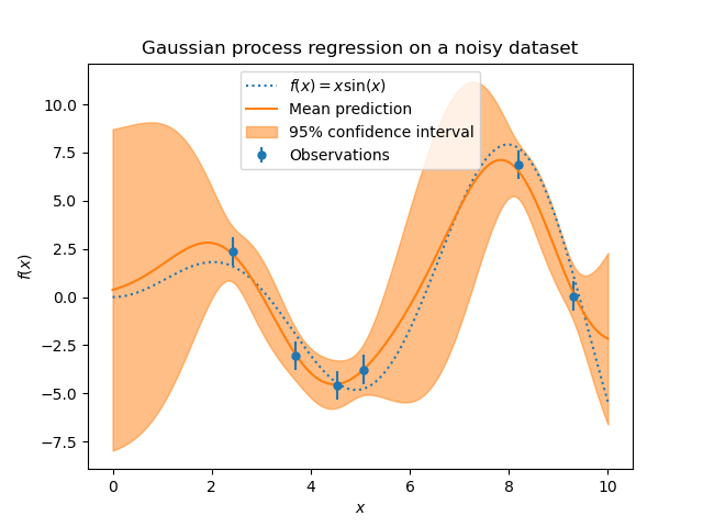
噪声会影响靠近训练样本的预测：由于我们明确地建模了一个与输入变量无关的给定水平目标噪声，因此靠近训练样本的预测不确定性更大。

脚本总运行时间： (0 分钟 0.486 秒)

高斯过程回归：基本入门示例#

数据集生成#

无噪声目标示例#

有噪声目标示例#

本页