注意
跳到文末下载完整的示例代码,或通过 JupyterLite 或 Binder 在浏览器中运行此示例。
核岭回归与高斯过程回归的比较#
本示例说明了核岭回归和高斯过程回归之间的差异。
核岭回归和高斯过程回归都使用了所谓的“核技巧”来使它们的模型具有足够的表达能力来拟合训练数据。然而,这两种方法解决的机器学习问题却截然不同。
核岭回归将找到使损失函数(均方误差)最小化的目标函数。
高斯过程回归不是寻找单一目标函数,而是采用概率方法:基于贝叶斯定理定义了目标函数的高斯后验分布。因此,目标函数的先验概率与由观测训练数据定义的似然函数相结合,以提供后验分布的估计。
我们将通过一个示例来说明这些差异,并将重点放在核超参数的调优上。
# Authors: The scikit-learn developers
# SPDX-License-Identifier: BSD-3-Clause
生成数据集#
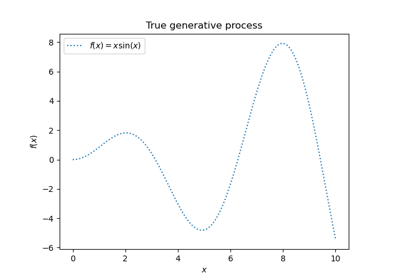
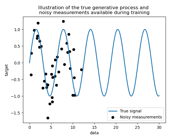
我们创建一个合成数据集。真实的生成过程将接收一个一维向量并计算其正弦值。请注意,此正弦的周期因此为 \(2 \pi\)。我们将在本示例的后面部分重用此信息。
import numpy as np

rng = np.random.RandomState(0)
data = np.linspace(0, 30, num=1_000).reshape(-1, 1)
target = np.sin(data).ravel()
现在,我们可以想象一个从真实过程获得观测值的场景。但是,我们会增加一些挑战:
测量结果会带有噪声;
只有信号开始部分的样本可用。
training_sample_indices = rng.choice(np.arange(0, 400), size=40, replace=False)
training_data = data[training_sample_indices]
training_noisy_target = target[training_sample_indices] + 0.5 * rng.randn(
    len(training_sample_indices)
)
让我们绘制真实信号和可用于训练的带噪声测量结果。
import matplotlib.pyplot as plt

plt.plot(data, target, label="True signal", linewidth=2)
plt.scatter(
    training_data,
    training_noisy_target,
    color="black",
    label="Noisy measurements",
)
plt.legend()
plt.xlabel("data")
plt.ylabel("target")
_ = plt.title(
    "Illustration of the true generative process and \n"
    "noisy measurements available during training"
)
简单线性模型的局限性#
首先,我们想强调给定数据集的线性模型的局限性。我们拟合一个 Ridge 模型,并检查该模型在我们数据集上的预测。
from sklearn.linear_model import Ridge

ridge = Ridge().fit(training_data, training_noisy_target)

plt.plot(data, target, label="True signal", linewidth=2)
plt.scatter(
    training_data,
    training_noisy_target,
    color="black",
    label="Noisy measurements",
)
plt.plot(data, ridge.predict(data), label="Ridge regression")
plt.legend()
plt.xlabel("data")
plt.ylabel("target")
_ = plt.title("Limitation of a linear model such as ridge")
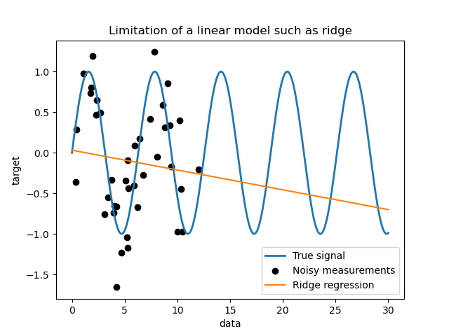
这样的岭回归器欠拟合数据,因为它表达能力不足。
核方法:核岭回归和高斯过程#
核岭回归#
我们可以通过使用所谓的核来使先前的线性模型更具表达能力。核是从原始特征空间到另一个特征空间的嵌入。简单来说,它用于将我们的原始数据映射到更新、更复杂的特征空间。这个新空间由核的选择明确定义。
在我们的案例中,我们知道真实的生成过程是一个周期函数。我们可以使用一个 ExpSineSquared 核,它允许恢复周期性。 KernelRidge 类将接受这样的核。
将此模型与核一起使用,相当于使用核的映射函数嵌入数据,然后应用岭回归。实际上,数据不会显式映射;而是使用“核技巧”计算高维特征空间中样本之间的点积。
因此,让我们使用这样的 KernelRidge 模型。
import time

from sklearn.gaussian_process.kernels import ExpSineSquared
from sklearn.kernel_ridge import KernelRidge

kernel_ridge = KernelRidge(kernel=ExpSineSquared())

start_time = time.time()
kernel_ridge.fit(training_data, training_noisy_target)
print(
    f"Fitting KernelRidge with default kernel: {time.time() - start_time:.3f} seconds"
)
Fitting KernelRidge with default kernel: 0.001 seconds
plt.plot(data, target, label="True signal", linewidth=2, linestyle="dashed")
plt.scatter(
    training_data,
    training_noisy_target,
    color="black",
    label="Noisy measurements",
)
plt.plot(
    data,
    kernel_ridge.predict(data),
    label="Kernel ridge",
    linewidth=2,
    linestyle="dashdot",
)
plt.legend(loc="lower right")
plt.xlabel("data")
plt.ylabel("target")
_ = plt.title(
    "Kernel ridge regression with an exponential sine squared\n "
    "kernel using default hyperparameters"
)
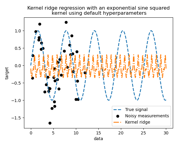
这个拟合的模型不准确。事实上,我们没有设置核的参数,而是使用了默认参数。我们可以检查它们。
kernel_ridge.kernel
ExpSineSquared(length_scale=1, periodicity=1)
我们的核有两个参数:长度尺度(length-scale)和周期性(periodicity)。对于我们的数据集,我们使用 sin 作为生成过程,这意味着信号具有 \(2 \pi\) 的周期性。参数的默认值为 \(1\),这解释了我们的模型预测中观察到的高频。对于长度尺度参数也可以得出类似的结论。因此,这告诉我们核参数需要进行调优。我们将使用随机搜索来调优核岭模型中的不同参数:alpha 参数和核参数。
from scipy.stats import loguniform

from sklearn.model_selection import RandomizedSearchCV

param_distributions = {
    "alpha": loguniform(1e0, 1e3),
    "kernel__length_scale": loguniform(1e-2, 1e2),
    "kernel__periodicity": loguniform(1e0, 1e1),
}
kernel_ridge_tuned = RandomizedSearchCV(
    kernel_ridge,
    param_distributions=param_distributions,
    n_iter=500,
    random_state=0,
)
start_time = time.time()
kernel_ridge_tuned.fit(training_data, training_noisy_target)
print(f"Time for KernelRidge fitting: {time.time() - start_time:.3f} seconds")
Time for KernelRidge fitting: 3.697 seconds
现在拟合模型的计算成本更高,因为我们必须尝试超参数的多种组合。我们可以查看找到的超参数以获得一些直观的理解。
kernel_ridge_tuned.best_params_
{'alpha': np.float64(1.991584977345022), 'kernel__length_scale': np.float64(0.7986499491396734), 'kernel__periodicity': np.float64(6.6072758064261095)}
查看最佳参数,我们发现它们与默认参数不同。我们还看到周期性更接近预期值:\(2 \pi\)。现在我们可以检查已调优核岭回归的预测。
Time for KernelRidge predict: 0.001 seconds
plt.plot(data, target, label="True signal", linewidth=2, linestyle="dashed")
plt.scatter(
    training_data,
    training_noisy_target,
    color="black",
    label="Noisy measurements",
)
plt.plot(
    data,
    predictions_kr,
    label="Kernel ridge",
    linewidth=2,
    linestyle="dashdot",
)
plt.legend(loc="lower right")
plt.xlabel("data")
plt.ylabel("target")
_ = plt.title(
    "Kernel ridge regression with an exponential sine squared\n "
    "kernel using tuned hyperparameters"
)
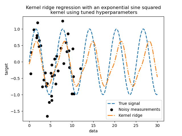
我们得到了一个更精确的模型。我们仍然观察到一些误差,主要是由于数据集中添加了噪声。
高斯过程回归#
现在,我们将使用 GaussianProcessRegressor 来拟合相同的数据集。在训练高斯过程时,核的超参数会在拟合过程中进行优化。不需要外部超参数搜索。在这里,我们创建了一个比核岭回归器稍微复杂的核:我们添加了一个 WhiteKernel,用于估计数据集中的噪声。
from sklearn.gaussian_process import GaussianProcessRegressor
from sklearn.gaussian_process.kernels import WhiteKernel

kernel = 1.0 * ExpSineSquared(1.0, 5.0, periodicity_bounds=(1e-2, 1e1)) + WhiteKernel(
    1e-1
)
gaussian_process = GaussianProcessRegressor(kernel=kernel)
start_time = time.time()
gaussian_process.fit(training_data, training_noisy_target)
print(
    f"Time for GaussianProcessRegressor fitting: {time.time() - start_time:.3f} seconds"
)
Time for GaussianProcessRegressor fitting: 0.030 seconds
训练高斯过程的计算成本远低于使用随机搜索的核岭回归。我们可以检查我们计算出的核的参数。
gaussian_process.kernel_
0.675**2 * ExpSineSquared(length_scale=1.34, periodicity=6.57) + WhiteKernel(noise_level=0.182)
确实,我们看到参数已经被优化了。查看 periodicity 参数,我们发现其周期接近理论值 \(2 \pi\)。现在我们可以看看模型的预测结果了。
Time for GaussianProcessRegressor predict: 0.002 seconds
plt.plot(data, target, label="True signal", linewidth=2, linestyle="dashed")
plt.scatter(
    training_data,
    training_noisy_target,
    color="black",
    label="Noisy measurements",
)
# Plot the predictions of the kernel ridge
plt.plot(
    data,
    predictions_kr,
    label="Kernel ridge",
    linewidth=2,
    linestyle="dashdot",
)
# Plot the predictions of the gaussian process regressor
plt.plot(
    data,
    mean_predictions_gpr,
    label="Gaussian process regressor",
    linewidth=2,
    linestyle="dotted",
)
plt.fill_between(
    data.ravel(),
    mean_predictions_gpr - std_predictions_gpr,
    mean_predictions_gpr + std_predictions_gpr,
    color="tab:green",
    alpha=0.2,
)
plt.legend(loc="lower right")
plt.xlabel("data")
plt.ylabel("target")
_ = plt.title("Comparison between kernel ridge and gaussian process regressor")
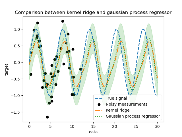
我们观察到核岭回归和高斯过程回归的结果非常接近。然而,高斯过程回归还提供了不确定性信息,这是核岭回归无法提供的。由于目标函数的概率公式,高斯过程可以输出标准差(或协方差)以及目标函数的平均预测。
然而,这也有代价:高斯过程的预测计算时间更长。
最终结论#
关于这两种模型的外推能力,我们可以给出最后一点说明。实际上,我们仅提供了信号的开头作为训练集。使用周期核迫使我们的模型重复在训练集上找到的模式。结合这种核信息以及两种模型的外推能力,我们观察到模型将继续预测正弦模式。
高斯过程允许将多个核组合在一起。因此,我们可以将指数正弦平方核与径向基函数核关联起来。
from sklearn.gaussian_process.kernels import RBF

kernel = 1.0 * ExpSineSquared(1.0, 5.0, periodicity_bounds=(1e-2, 1e1)) * RBF(
    length_scale=15, length_scale_bounds="fixed"
) + WhiteKernel(1e-1)
gaussian_process = GaussianProcessRegressor(kernel=kernel)
gaussian_process.fit(training_data, training_noisy_target)
mean_predictions_gpr, std_predictions_gpr = gaussian_process.predict(
    data,
    return_std=True,
)
plt.plot(data, target, label="True signal", linewidth=2, linestyle="dashed")
plt.scatter(
    training_data,
    training_noisy_target,
    color="black",
    label="Noisy measurements",
)
# Plot the predictions of the kernel ridge
plt.plot(
    data,
    predictions_kr,
    label="Kernel ridge",
    linewidth=2,
    linestyle="dashdot",
)
# Plot the predictions of the gaussian process regressor
plt.plot(
    data,
    mean_predictions_gpr,
    label="Gaussian process regressor",
    linewidth=2,
    linestyle="dotted",
)
plt.fill_between(
    data.ravel(),
    mean_predictions_gpr - std_predictions_gpr,
    mean_predictions_gpr + std_predictions_gpr,
    color="tab:green",
    alpha=0.2,
)
plt.legend(loc="lower right")
plt.xlabel("data")
plt.ylabel("target")
_ = plt.title("Effect of using a radial basis function kernel")
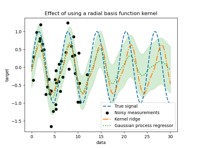
一旦训练中没有样本可用,使用径向基函数核的效果将减弱周期性效应。随着测试样本距离训练样本越来越远,预测会收敛到其均值,并且其标准差也会增加。
脚本总运行时间: (0 分钟 4.333 秒)
相关示例