注意
跳转到末尾 下载完整示例代码。或通过JupyterLite或Binder在浏览器中运行此示例
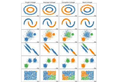
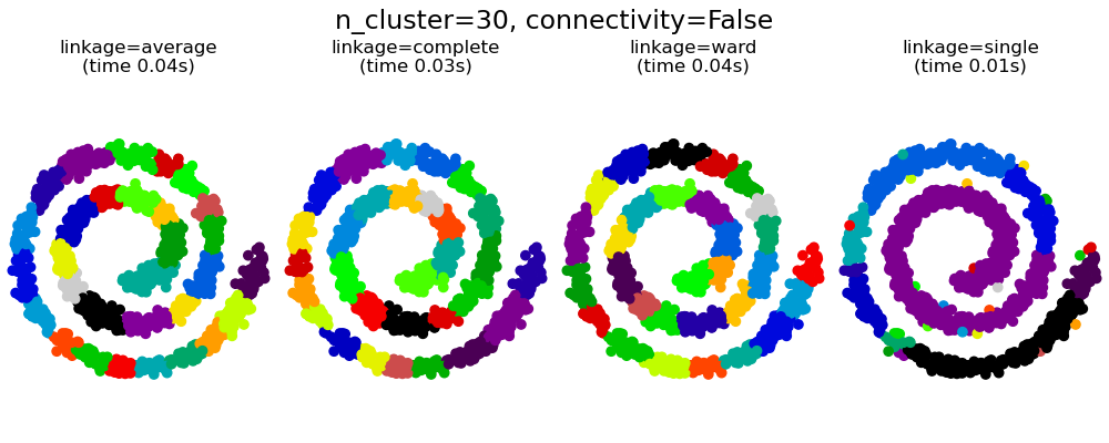
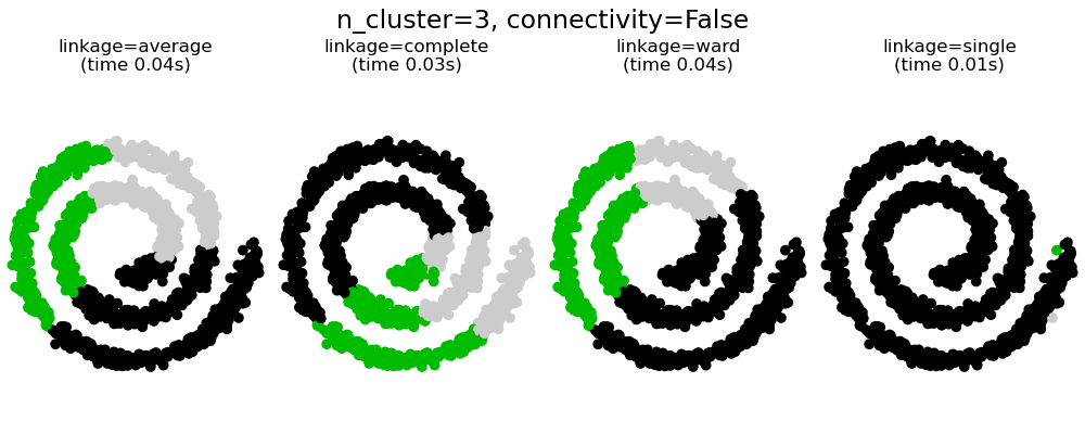
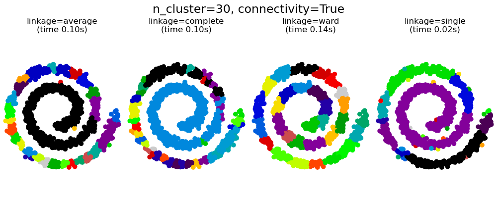
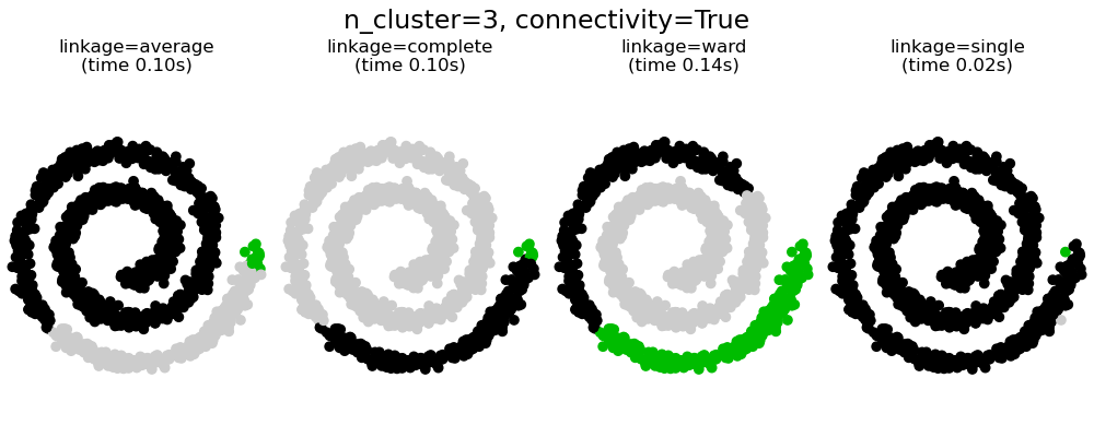
带结构和不带结构的凝聚聚类#
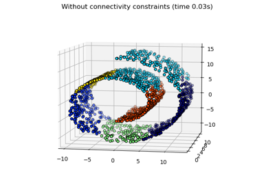
本示例展示了施加连接图来捕获数据中局部结构的效果。该图就是20个最近邻的图。
施加连接性有两个优点。首先,使用稀疏连接矩阵进行聚类通常更快。
其次,当使用连接矩阵时,单一、平均和完全链接是不稳定的,并且倾向于创建一些增长非常快的聚类。实际上,平均和完全链接通过在合并两个聚类时考虑它们之间的所有距离来对抗这种渗流行为(而单一链接通过仅考虑聚类之间最短的距离来夸大这种行为)。连接图打破了平均和完全链接的这种机制,使它们更像脆弱的单一链接。这种效应对于非常稀疏的图(尝试减少kneighbors_graph中的邻居数量)和完全链接更为明显。特别是,图中邻居数量非常少时,会形成一种接近单一链接的几何结构,而单一链接众所周知存在这种渗流不稳定性。
# Authors: The scikit-learn developers
# SPDX-License-Identifier: BSD-3-Clause

import time

import matplotlib.pyplot as plt
import numpy as np

from sklearn.cluster import AgglomerativeClustering
from sklearn.neighbors import kneighbors_graph

# Generate sample data
n_samples = 1500
np.random.seed(0)
t = 1.5 * np.pi * (1 + 3 * np.random.rand(1, n_samples))
x = t * np.cos(t)
y = t * np.sin(t)


X = np.concatenate((x, y))
X += 0.7 * np.random.randn(2, n_samples)
X = X.T

# Create a graph capturing local connectivity. Larger number of neighbors
# will give more homogeneous clusters to the cost of computation
# time. A very large number of neighbors gives more evenly distributed
# cluster sizes, but may not impose the local manifold structure of
# the data
knn_graph = kneighbors_graph(X, 30, include_self=False)

for connectivity in (None, knn_graph):
    for n_clusters in (30, 3):
        plt.figure(figsize=(10, 4))
        for index, linkage in enumerate(("average", "complete", "ward", "single")):
            plt.subplot(1, 4, index + 1)
            model = AgglomerativeClustering(
                linkage=linkage, connectivity=connectivity, n_clusters=n_clusters
            )
            t0 = time.time()
            model.fit(X)
            elapsed_time = time.time() - t0
            plt.scatter(X[:, 0], X[:, 1], c=model.labels_, cmap=plt.cm.nipy_spectral)
            plt.title(
                "linkage=%s\n(time %.2fs)" % (linkage, elapsed_time),
                fontdict=dict(verticalalignment="top"),
            )
            plt.axis("equal")
            plt.axis("off")

            plt.subplots_adjust(bottom=0, top=0.83, wspace=0, left=0, right=1)
            plt.suptitle(
                "n_cluster=%i, connectivity=%r"
                % (n_clusters, connectivity is not None),
                size=17,
            )


plt.show()
脚本总运行时间: (0 分钟 1.845 秒)
相关示例