手写数字的流形学习：局部线性嵌入、Isomap…#

我们将演示在数字数据集上的各种嵌入技术。

# Authors: The scikit-learn developers
# SPDX-License-Identifier: BSD-3-Clause

加载数字数据集#

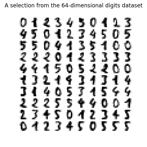
我们将加载数字数据集，并只使用十个可用类别中的前六个。

from sklearn.datasets import load_digits

digits = load_digits(n_class=6)
X, y = digits.data, digits.target
n_samples, n_features = X.shape
n_neighbors = 30

我们可以绘制该数据集的前一百个数字。

import matplotlib.pyplot as plt

fig, axs = plt.subplots(nrows=10, ncols=10, figsize=(6, 6))
for idx, ax in enumerate(axs.ravel()):
    ax.imshow(X[idx].reshape((8, 8)), cmap=plt.cm.binary)
    ax.axis("off")
_ = fig.suptitle("A selection from the 64-dimensional digits dataset", fontsize=16)

A selection from the 64-dimensional digits dataset

绘制嵌入的辅助函数#

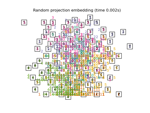
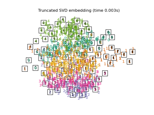
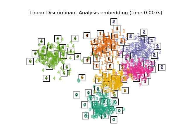
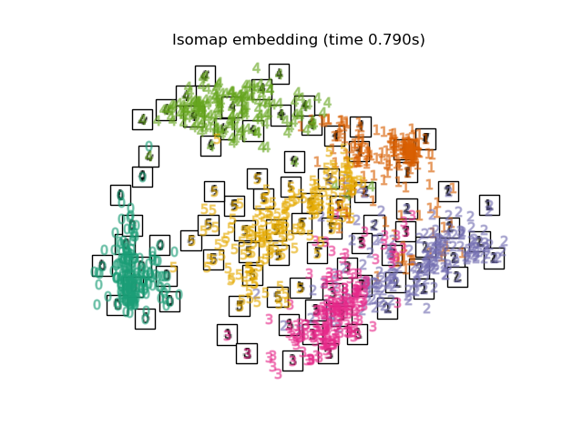
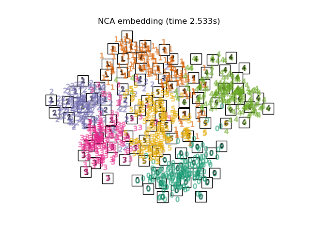
下面，我们将使用不同的技术嵌入数字数据集。我们将绘制原始数据在每个嵌入上的投影。这将使我们能够检查数字是否在嵌入空间中聚集在一起，或者是否散布开来。

import numpy as np
from matplotlib import offsetbox

from sklearn.preprocessing import MinMaxScaler


def plot_embedding(X, title):
    _, ax = plt.subplots()
    X = MinMaxScaler().fit_transform(X)

    for digit in digits.target_names:
        ax.scatter(
            *X[y == digit].T,
            marker=f"${digit}$",
            s=60,
            color=plt.cm.Dark2(digit),
            alpha=0.425,
            zorder=2,
        )
    shown_images = np.array([[1.0, 1.0]])  # just something big
    for i in range(X.shape[0]):
        # plot every digit on the embedding
        # show an annotation box for a group of digits
        dist = np.sum((X[i] - shown_images) ** 2, 1)
        if np.min(dist) < 4e-3:
            # don't show points that are too close
            continue
        shown_images = np.concatenate([shown_images, [X[i]]], axis=0)
        imagebox = offsetbox.AnnotationBbox(
            offsetbox.OffsetImage(digits.images[i], cmap=plt.cm.gray_r), X[i]
        )
        imagebox.set(zorder=1)
        ax.add_artist(imagebox)

    ax.set_title(title)
    ax.axis("off")

嵌入技术比较#

下面，我们比较了不同的技术。然而，有几点需要注意：

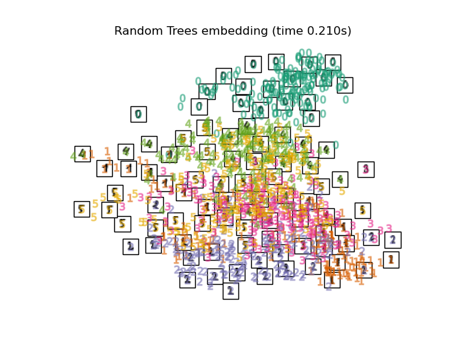
RandomTreesEmbedding 严格来说不是一种流形嵌入方法，因为它学习的是一个高维表示，然后我们在此表示上应用降维方法。然而，将数据集转换为类别可线性分离的表示通常很有用。
LinearDiscriminantAnalysis 和 NeighborhoodComponentsAnalysis 是监督降维方法，即它们利用了提供的标签，这与其他方法不同。
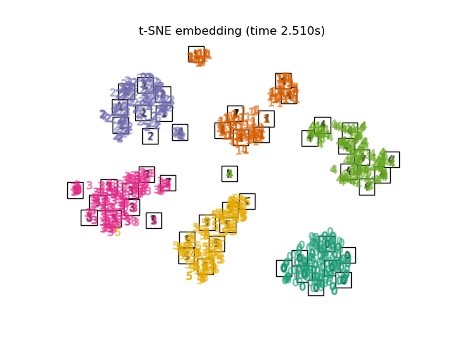
在本例中，TSNE 使用PCA生成的嵌入进行初始化。这确保了嵌入的全局稳定性，即嵌入不依赖于随机初始化。

from sklearn.decomposition import TruncatedSVD
from sklearn.discriminant_analysis import LinearDiscriminantAnalysis
from sklearn.ensemble import RandomTreesEmbedding
from sklearn.manifold import (
    MDS,
    TSNE,
    Isomap,
    LocallyLinearEmbedding,
    SpectralEmbedding,
)
from sklearn.neighbors import NeighborhoodComponentsAnalysis
from sklearn.pipeline import make_pipeline
from sklearn.random_projection import SparseRandomProjection

embeddings = {
    "Random projection embedding": SparseRandomProjection(
        n_components=2, random_state=42
    ),
    "Truncated SVD embedding": TruncatedSVD(n_components=2),
    "Linear Discriminant Analysis embedding": LinearDiscriminantAnalysis(
        n_components=2
    ),
    "Isomap embedding": Isomap(n_neighbors=n_neighbors, n_components=2),
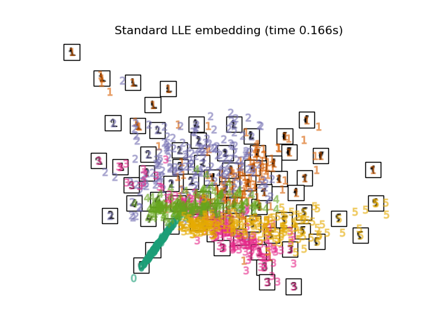
    "Standard LLE embedding": LocallyLinearEmbedding(
        n_neighbors=n_neighbors, n_components=2, method="standard"
    ),
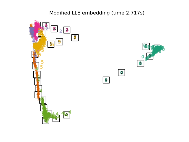
    "Modified LLE embedding": LocallyLinearEmbedding(
        n_neighbors=n_neighbors, n_components=2, method="modified"
    ),
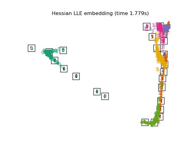
    "Hessian LLE embedding": LocallyLinearEmbedding(
        n_neighbors=n_neighbors, n_components=2, method="hessian"
    ),
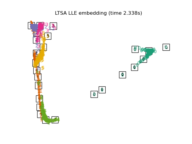
    "LTSA LLE embedding": LocallyLinearEmbedding(
        n_neighbors=n_neighbors, n_components=2, method="ltsa"
    ),
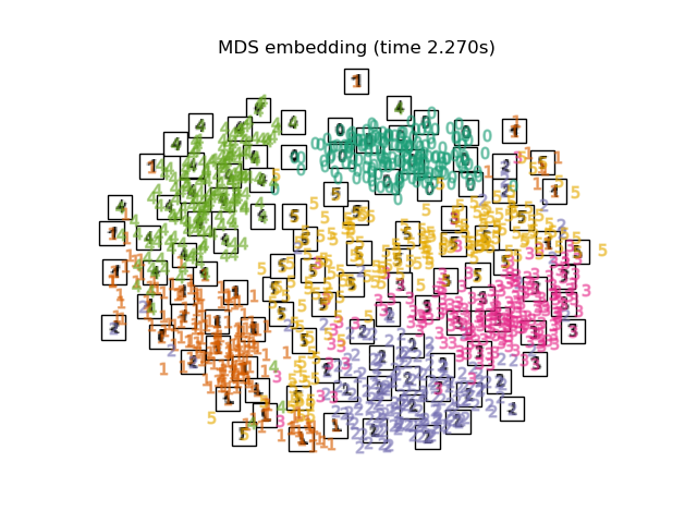
    "MDS embedding": MDS(n_components=2, n_init=1, max_iter=120, eps=1e-6),
    "Random Trees embedding": make_pipeline(
        RandomTreesEmbedding(n_estimators=200, max_depth=5, random_state=0),
        TruncatedSVD(n_components=2),
    ),
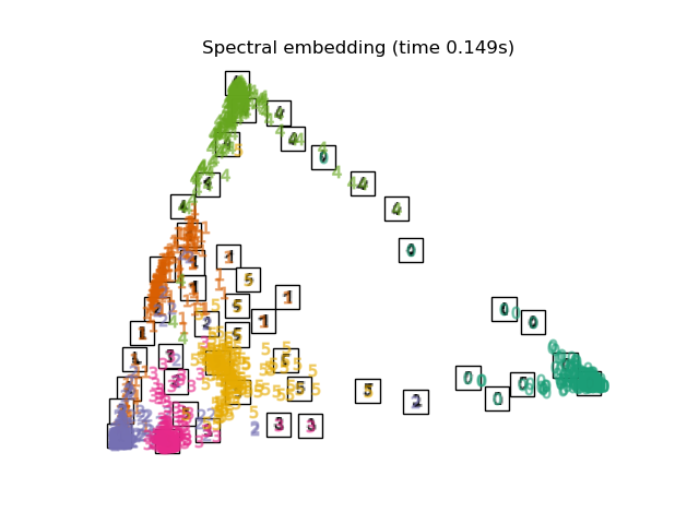
    "Spectral embedding": SpectralEmbedding(
        n_components=2, random_state=0, eigen_solver="arpack"
    ),
    "t-SNE embedding": TSNE(
        n_components=2,
        max_iter=500,
        n_iter_without_progress=150,
        n_jobs=2,
        random_state=0,
    ),
    "NCA embedding": NeighborhoodComponentsAnalysis(
        n_components=2, init="pca", random_state=0
    ),
}

声明所有感兴趣的方法后，我们可以运行并执行原始数据的投影。我们将存储投影数据以及执行每次投影所需的计算时间。

from time import time

projections, timing = {}, {}
for name, transformer in embeddings.items():
    if name.startswith("Linear Discriminant Analysis"):
        data = X.copy()
        data.flat[:: X.shape[1] + 1] += 0.01  # Make X invertible
    else:
        data = X

    print(f"Computing {name}...")
    start_time = time()
    projections[name] = transformer.fit_transform(data, y)
    timing[name] = time() - start_time

Computing Random projection embedding...
Computing Truncated SVD embedding...
Computing Linear Discriminant Analysis embedding...
Computing Isomap embedding...
Computing Standard LLE embedding...
Computing Modified LLE embedding...
Computing Hessian LLE embedding...
Computing LTSA LLE embedding...
Computing MDS embedding...
Computing Random Trees embedding...
Computing Spectral embedding...
Computing t-SNE embedding...
Computing NCA embedding...

最后，我们可以绘制每种方法给出的结果投影。

for name in timing:
    title = f"{name} (time {timing[name]:.3f}s)"
    plot_embedding(projections[name], title)

plt.show()

脚本总运行时间： (0 分钟 19.868 秒)

手写数字的流形学习：局部线性嵌入、Isomap…#

加载数字数据集#

绘制嵌入的辅助函数#

嵌入技术比较#

本页面