不同核函数下高斯过程的先验与后验示意图

本示例演示了不同核函数下 GaussianProcessRegressor 的先验和后验。先验和后验分布都显示了均值、标准差和 5 个样本。

此处仅作说明。要了解更多关于核函数公式的信息，请参阅用户指南。

# Authors: The scikit-learn developers
# SPDX-License-Identifier: BSD-3-Clause

辅助函数

在介绍高斯过程可用的每个独立核函数之前，我们将定义一个辅助函数，该函数允许我们绘制从高斯过程中抽取的样本。

此函数将接受一个 GaussianProcessRegressor 模型，并从高斯过程中抽取样本。如果模型未拟合，则样本从先验分布中抽取；模型拟合后，样本从后验分布中抽取。

import matplotlib.pyplot as plt
import numpy as np


def plot_gpr_samples(gpr_model, n_samples, ax):
    """Plot samples drawn from the Gaussian process model.

    If the Gaussian process model is not trained then the drawn samples are
    drawn from the prior distribution. Otherwise, the samples are drawn from
    the posterior distribution. Be aware that a sample here corresponds to a
    function.

    Parameters
    ----------
    gpr_model : `GaussianProcessRegressor`
        A :class:`~sklearn.gaussian_process.GaussianProcessRegressor` model.
    n_samples : int
        The number of samples to draw from the Gaussian process distribution.
    ax : matplotlib axis
        The matplotlib axis where to plot the samples.
    """
    x = np.linspace(0, 5, 100)
    X = x.reshape(-1, 1)

    y_mean, y_std = gpr_model.predict(X, return_std=True)
    y_samples = gpr_model.sample_y(X, n_samples)

    for idx, single_prior in enumerate(y_samples.T):
        ax.plot(
            x,
            single_prior,
            linestyle="--",
            alpha=0.7,
            label=f"Sampled function #{idx + 1}",
        )
    ax.plot(x, y_mean, color="black", label="Mean")
    ax.fill_between(
        x,
        y_mean - y_std,
        y_mean + y_std,
        alpha=0.1,
        color="black",
        label=r"$\pm$ 1 std. dev.",
    )
    ax.set_xlabel("x")
    ax.set_ylabel("y")
    ax.set_ylim([-3, 3])

数据集和高斯过程生成

我们将创建一个训练数据集，并在不同部分中使用它。

rng = np.random.RandomState(4)
X_train = rng.uniform(0, 5, 10).reshape(-1, 1)
y_train = np.sin((X_train[:, 0] - 2.5) ** 2)
n_samples = 5

核函数教程

在本节中，我们将演示从具有不同核函数的高斯过程的先验和后验分布中抽取的一些样本。

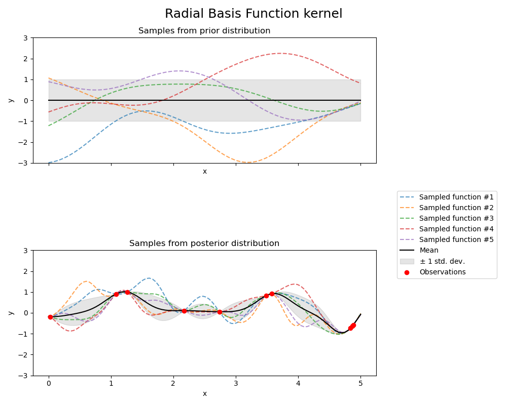
径向基函数核

from sklearn.gaussian_process import GaussianProcessRegressor
from sklearn.gaussian_process.kernels import RBF

kernel = 1.0 * RBF(length_scale=1.0, length_scale_bounds=(1e-1, 10.0))
gpr = GaussianProcessRegressor(kernel=kernel, random_state=0)

fig, axs = plt.subplots(nrows=2, sharex=True, sharey=True, figsize=(10, 8))

# plot prior
plot_gpr_samples(gpr, n_samples=n_samples, ax=axs[0])
axs[0].set_title("Samples from prior distribution")

# plot posterior
gpr.fit(X_train, y_train)
plot_gpr_samples(gpr, n_samples=n_samples, ax=axs[1])
axs[1].scatter(X_train[:, 0], y_train, color="red", zorder=10, label="Observations")
axs[1].legend(bbox_to_anchor=(1.05, 1.5), loc="upper left")
axs[1].set_title("Samples from posterior distribution")

fig.suptitle("Radial Basis Function kernel", fontsize=18)
plt.tight_layout()

print(f"Kernel parameters before fit:\n{kernel})")
print(
    f"Kernel parameters after fit: \n{gpr.kernel_} \n"
    f"Log-likelihood: {gpr.log_marginal_likelihood(gpr.kernel_.theta):.3f}"
)

Kernel parameters before fit:
1**2 * RBF(length_scale=1))
Kernel parameters after fit:
0.594**2 * RBF(length_scale=0.279)
Log-likelihood: -0.067

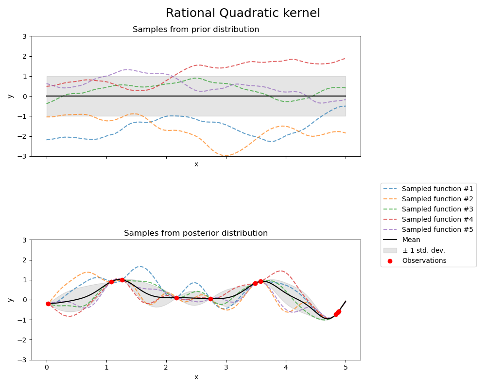
有理二次核

from sklearn.gaussian_process.kernels import RationalQuadratic

kernel = 1.0 * RationalQuadratic(length_scale=1.0, alpha=0.1, alpha_bounds=(1e-5, 1e15))
gpr = GaussianProcessRegressor(kernel=kernel, random_state=0)

fig, axs = plt.subplots(nrows=2, sharex=True, sharey=True, figsize=(10, 8))

# plot prior
plot_gpr_samples(gpr, n_samples=n_samples, ax=axs[0])
axs[0].set_title("Samples from prior distribution")

# plot posterior
gpr.fit(X_train, y_train)
plot_gpr_samples(gpr, n_samples=n_samples, ax=axs[1])
axs[1].scatter(X_train[:, 0], y_train, color="red", zorder=10, label="Observations")
axs[1].legend(bbox_to_anchor=(1.05, 1.5), loc="upper left")
axs[1].set_title("Samples from posterior distribution")

fig.suptitle("Rational Quadratic kernel", fontsize=18)
plt.tight_layout()

print(f"Kernel parameters before fit:\n{kernel})")
print(
    f"Kernel parameters after fit: \n{gpr.kernel_} \n"
    f"Log-likelihood: {gpr.log_marginal_likelihood(gpr.kernel_.theta):.3f}"
)

Kernel parameters before fit:
1**2 * RationalQuadratic(alpha=0.1, length_scale=1))
Kernel parameters after fit:
0.594**2 * RationalQuadratic(alpha=1.73e+06, length_scale=0.279)
Log-likelihood: -0.067

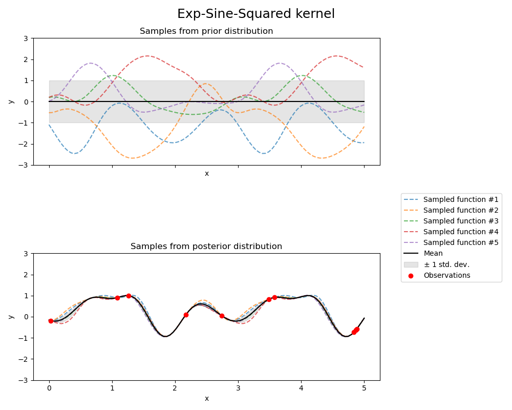
指数正弦平方核

from sklearn.gaussian_process.kernels import ExpSineSquared

kernel = 1.0 * ExpSineSquared(
    length_scale=1.0,
    periodicity=3.0,
    length_scale_bounds=(0.1, 10.0),
    periodicity_bounds=(1.0, 10.0),
)
gpr = GaussianProcessRegressor(kernel=kernel, random_state=0)

fig, axs = plt.subplots(nrows=2, sharex=True, sharey=True, figsize=(10, 8))

# plot prior
plot_gpr_samples(gpr, n_samples=n_samples, ax=axs[0])
axs[0].set_title("Samples from prior distribution")

# plot posterior
gpr.fit(X_train, y_train)
plot_gpr_samples(gpr, n_samples=n_samples, ax=axs[1])
axs[1].scatter(X_train[:, 0], y_train, color="red", zorder=10, label="Observations")
axs[1].legend(bbox_to_anchor=(1.05, 1.5), loc="upper left")
axs[1].set_title("Samples from posterior distribution")

fig.suptitle("Exp-Sine-Squared kernel", fontsize=18)
plt.tight_layout()

print(f"Kernel parameters before fit:\n{kernel})")
print(
    f"Kernel parameters after fit: \n{gpr.kernel_} \n"
    f"Log-likelihood: {gpr.log_marginal_likelihood(gpr.kernel_.theta):.3f}"
)

Kernel parameters before fit:
1**2 * ExpSineSquared(length_scale=1, periodicity=3))
Kernel parameters after fit:
0.799**2 * ExpSineSquared(length_scale=0.791, periodicity=2.87)
Log-likelihood: 3.394

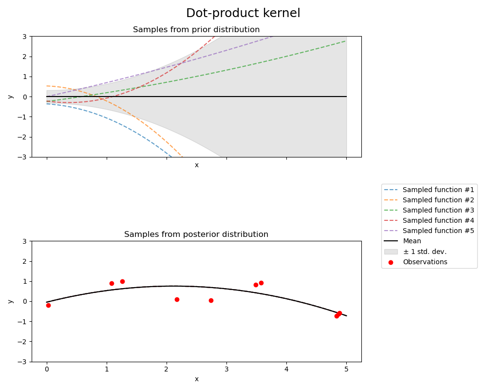
点积核

from sklearn.gaussian_process.kernels import ConstantKernel, DotProduct

kernel = ConstantKernel(0.1, (0.01, 10.0)) * (
    DotProduct(sigma_0=1.0, sigma_0_bounds=(0.1, 10.0)) ** 2
)
gpr = GaussianProcessRegressor(kernel=kernel, random_state=0, normalize_y=True)

fig, axs = plt.subplots(nrows=2, sharex=True, sharey=True, figsize=(10, 8))

# plot prior
plot_gpr_samples(gpr, n_samples=n_samples, ax=axs[0])
axs[0].set_title("Samples from prior distribution")

# plot posterior
gpr.fit(X_train, y_train)
plot_gpr_samples(gpr, n_samples=n_samples, ax=axs[1])
axs[1].scatter(X_train[:, 0], y_train, color="red", zorder=10, label="Observations")
axs[1].legend(bbox_to_anchor=(1.05, 1.5), loc="upper left")
axs[1].set_title("Samples from posterior distribution")

fig.suptitle("Dot-product kernel", fontsize=18)
plt.tight_layout()

print(f"Kernel parameters before fit:\n{kernel})")
print(
    f"Kernel parameters after fit: \n{gpr.kernel_} \n"
    f"Log-likelihood: {gpr.log_marginal_likelihood(gpr.kernel_.theta):.3f}"
)

Kernel parameters before fit:
0.316**2 * DotProduct(sigma_0=1) ** 2)
Kernel parameters after fit:
0.697**2 * DotProduct(sigma_0=0.454) ** 2
Log-likelihood: -18108182014.707

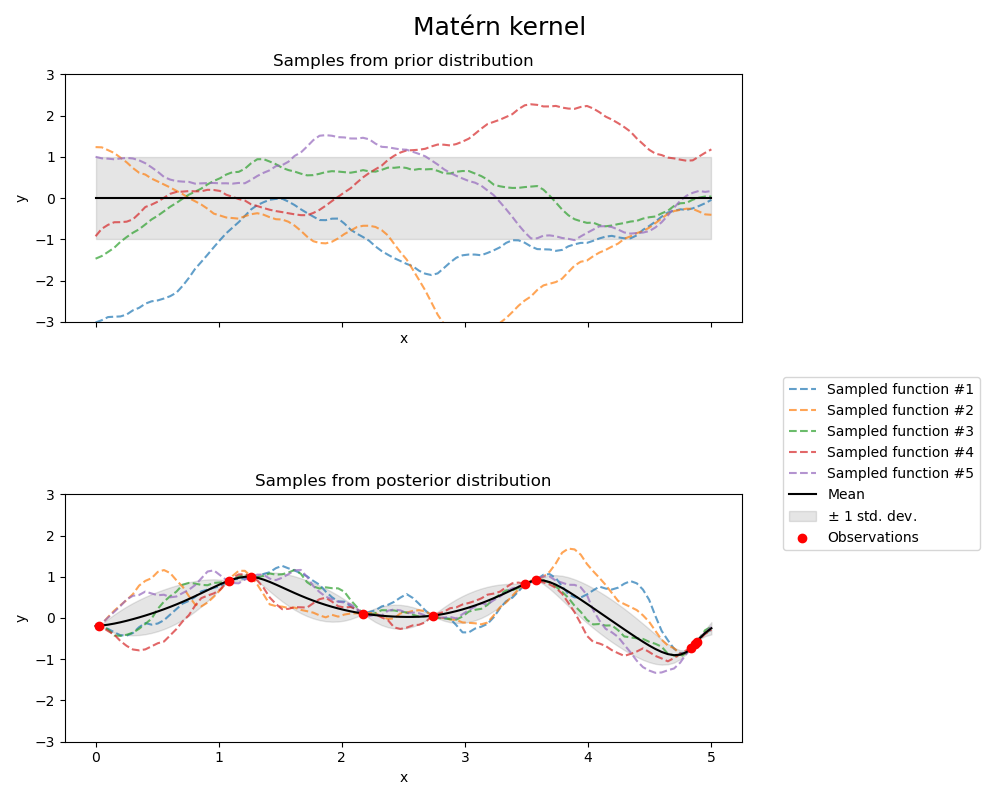
Matérn 核

from sklearn.gaussian_process.kernels import Matern

kernel = 1.0 * Matern(length_scale=1.0, length_scale_bounds=(1e-1, 10.0), nu=1.5)
gpr = GaussianProcessRegressor(kernel=kernel, random_state=0)

fig, axs = plt.subplots(nrows=2, sharex=True, sharey=True, figsize=(10, 8))

# plot prior
plot_gpr_samples(gpr, n_samples=n_samples, ax=axs[0])
axs[0].set_title("Samples from prior distribution")

# plot posterior
gpr.fit(X_train, y_train)
plot_gpr_samples(gpr, n_samples=n_samples, ax=axs[1])
axs[1].scatter(X_train[:, 0], y_train, color="red", zorder=10, label="Observations")
axs[1].legend(bbox_to_anchor=(1.05, 1.5), loc="upper left")
axs[1].set_title("Samples from posterior distribution")

fig.suptitle("Matérn kernel", fontsize=18)
plt.tight_layout()

print(f"Kernel parameters before fit:\n{kernel})")
print(
    f"Kernel parameters after fit: \n{gpr.kernel_} \n"
    f"Log-likelihood: {gpr.log_marginal_likelihood(gpr.kernel_.theta):.3f}"
)

Kernel parameters before fit:
1**2 * Matern(length_scale=1, nu=1.5))
Kernel parameters after fit:
0.609**2 * Matern(length_scale=0.484, nu=1.5)
Log-likelihood: -1.185

相关示例

高斯过程回归 (GPR) 估计数据噪声水平的能力

高斯过程回归 (GPR) 估计数据噪声水平的能力

k-均值假设的演示

k-均值假设的演示

二分 K-均值与常规 K-均值性能比较

二分 K-均值与常规 K-均值性能比较

高斯过程回归：基本介绍示例

高斯过程回归：基本介绍示例