注意
跳转到末尾 下载完整示例代码,或通过 JupyterLite 或 Binder 在浏览器中运行此示例
线性模型系数解释中的常见陷阱#
在线性模型中,目标值被建模为特征的线性组合(请参阅 线性模型 用户指南部分,了解 scikit-learn 中可用的一组线性模型的描述)。多元线性模型中的系数表示给定特征 \(X_i\) 与目标 \(y\) 之间的关系,前提是所有其他特征保持不变(条件依赖性)。这与绘制 \(X_i\) 对 \(y\) 并拟合线性关系不同:在后一种情况下,估计中考虑了其他特征的所有可能值(边际依赖性)。
本示例将提供一些解释线性模型系数的提示,指出当线性模型不适合描述数据集或特征相关时出现的问题。
注意
请记住,特征 \(X\) 和结果 \(y\) 通常是数据生成过程的产物,而该过程对我们来说是未知的。机器学习模型经过训练,旨在从样本数据中近似连接 \(X\) 到 \(y\) 的未观测数学函数。因此,对模型所做的任何解释不一定能推广到真实的数据生成过程。当模型质量不佳或样本数据不具有代表性时,尤其如此。
我们将使用 1985 年 “当前人口调查” 的数据,根据经验、年龄或教育等各种特征来预测工资。
# Authors: The scikit-learn developers
# SPDX-License-Identifier: BSD-3-Clause
import matplotlib.pyplot as plt
import numpy as np
import pandas as pd
import scipy as sp
import seaborn as sns
数据集:工资#
我们从 OpenML 获取数据。请注意,将参数 as_frame 设置为 True 将把数据检索为 pandas 数据框。
from sklearn.datasets import fetch_openml

survey = fetch_openml(data_id=534, as_frame=True)
然后,我们识别特征 X 和目标 y:WAGE 列是我们的目标变量(即我们想要预测的变量)。
X = survey.data[survey.feature_names]
X.describe(include="all")
请注意,数据集包含分类变量和数值变量。我们随后在预处理数据集时需要考虑到这一点。
X.head()
我们的预测目标:工资。工资被描述为每小时美元的浮点数。
y = survey.target.values.ravel()
survey.target.head()
0    5.10
1    4.95
2    6.67
3    4.00
4    7.50
Name: WAGE, dtype: float64
我们将样本拆分为训练数据集和测试数据集。在接下来的探索性分析中,只使用训练数据集。这是一种模拟真实情况的方法,即在未知目标上执行预测,我们不希望我们的分析和决策受到对测试数据了解的偏见。
from sklearn.model_selection import train_test_split

X_train, X_test, y_train, y_test = train_test_split(X, y, random_state=42)
首先,让我们通过查看变量分布和它们之间的成对关系来获得一些见解。只使用数值变量。在下图中,每个点代表一个样本。
train_dataset = X_train.copy()
train_dataset.insert(0, "WAGE", y_train)
_ = sns.pairplot(train_dataset, kind="reg", diag_kind="kde")
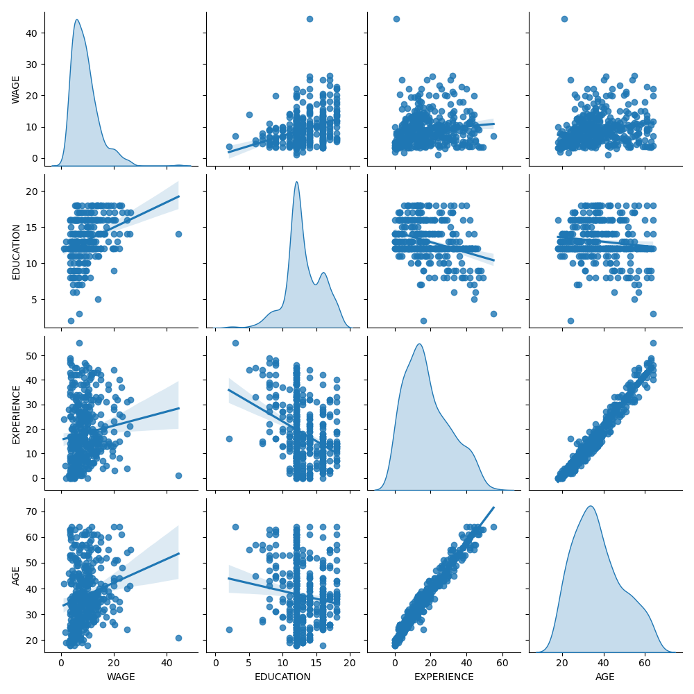
仔细观察工资(WAGE)分布,会发现它有一个长尾。因此,我们应该取其对数,使其近似为正态分布(岭回归或 Lasso 等线性模型最适合误差的正态分布)。
当教育水平(EDUCATION)提高时,工资(WAGE)也会增加。请注意,此处表示的工资与教育之间的依赖性是边际依赖性,即它描述了特定变量的行为,而没有保持其他变量固定。
此外,经验(EXPERIENCE)和年龄(AGE)之间存在强线性相关。
机器学习流水线#
为了设计我们的机器学习流水线,我们首先手动检查正在处理的数据类型
survey.data.info()
<class 'pandas.core.frame.DataFrame'>
RangeIndex: 534 entries, 0 to 533
Data columns (total 10 columns):
 #   Column      Non-Null Count  Dtype
---  ------      --------------  -----
 0   EDUCATION   534 non-null    int64
 1   SOUTH       534 non-null    category
 2   SEX         534 non-null    category
 3   EXPERIENCE  534 non-null    int64
 4   UNION       534 non-null    category
 5   AGE         534 non-null    int64
 6   RACE        534 non-null    category
 7   OCCUPATION  534 non-null    category
 8   SECTOR      534 non-null    category
 9   MARR        534 non-null    category
dtypes: category(7), int64(3)
memory usage: 17.2 KB
如前所述,数据集包含具有不同数据类型的列,我们需要对每种数据类型应用特定的预处理。特别是,如果分类变量未首先编码为整数,则无法将其包含在线性模型中。此外,为避免将分类特征视为有序值,我们需要对其进行独热编码。我们的预处理器将:
对分类列进行独热编码(即按类别生成一列),仅适用于非二元分类变量;
作为第一种方法(我们稍后将看到数值的归一化将如何影响我们的讨论),保持数值不变。
from sklearn.compose import make_column_transformer
from sklearn.preprocessing import OneHotEncoder

categorical_columns = ["RACE", "OCCUPATION", "SECTOR", "MARR", "UNION", "SEX", "SOUTH"]
numerical_columns = ["EDUCATION", "EXPERIENCE", "AGE"]

preprocessor = make_column_transformer(
    (OneHotEncoder(drop="if_binary"), categorical_columns),
    remainder="passthrough",
    verbose_feature_names_out=False,  # avoid to prepend the preprocessor names
)
为了将数据集描述为线性模型,我们使用具有非常小正则化的岭回归器,并对工资(WAGE)的对数进行建模。
from sklearn.compose import TransformedTargetRegressor
from sklearn.linear_model import Ridge
from sklearn.pipeline import make_pipeline

model = make_pipeline(
    preprocessor,
    TransformedTargetRegressor(
        regressor=Ridge(alpha=1e-10), func=np.log10, inverse_func=sp.special.exp10
    ),
)
处理数据集#
首先,我们拟合模型。
model.fit(X_train, y_train)
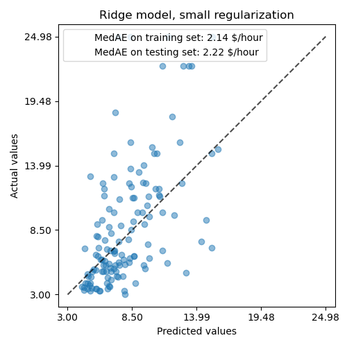
然后,我们通过绘制其在测试集上的预测并计算例如模型的中间绝对误差来检查计算模型的性能。
from sklearn.metrics import PredictionErrorDisplay, median_absolute_error

mae_train = median_absolute_error(y_train, model.predict(X_train))
y_pred = model.predict(X_test)
mae_test = median_absolute_error(y_test, y_pred)
scores = {
    "MedAE on training set": f"{mae_train:.2f} $/hour",
    "MedAE on testing set": f"{mae_test:.2f} $/hour",
}
_, ax = plt.subplots(figsize=(5, 5))
display = PredictionErrorDisplay.from_predictions(
    y_test, y_pred, kind="actual_vs_predicted", ax=ax, scatter_kwargs={"alpha": 0.5}
)
ax.set_title("Ridge model, small regularization")
for name, score in scores.items():
    ax.plot([], [], " ", label=f"{name}: {score}")
ax.legend(loc="upper left")
plt.tight_layout()

所学习的模型远不是一个能做出准确预测的好模型:从上图可以看出这一点,其中好的预测应该落在黑色虚线上。
在下一节中,我们将解释模型的系数。在此过程中,我们应该记住,我们得出的任何结论都只与我们构建的模型有关,而不是关于数据的真实(现实世界)生成过程。
解释系数:尺度很重要#
首先,我们可以查看我们已拟合的回归器的系数值。
feature_names = model[:-1].get_feature_names_out()

coefs = pd.DataFrame(
    model[-1].regressor_.coef_,
    columns=["Coefficients"],
    index=feature_names,
)

coefs
年龄(AGE)系数表示为“美元/小时/生活年”,而教育(EDUCATION)系数表示为“美元/小时/教育年”。这种系数表示的优点在于清楚地揭示了模型的实际预测:年龄增加 \(1\) 年意味着每小时工资减少 \(0.030867\) 美元,而教育增加 \(1\) 年意味着每小时工资增加 \(0.054699\) 美元。另一方面,分类变量(如工会 UNION 或性别 SEX)是无量纲数,取值 0 或 1。它们的系数以美元/小时表示。因此,我们无法比较不同系数的大小,因为这些特征具有不同的自然尺度和值范围,这是由于它们具有不同的计量单位。如果我们绘制系数,这一点会更加明显。
coefs.plot.barh(figsize=(9, 7))
plt.title("Ridge model, small regularization")
plt.axvline(x=0, color=".5")
plt.xlabel("Raw coefficient values")
plt.subplots_adjust(left=0.3)
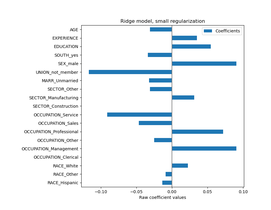
事实上,从上图中,决定工资(WAGE)的最重要因素似乎是变量 UNION,即使我们的直觉可能告诉我们像经验(EXPERIENCE)这样的变量应该有更大的影响。
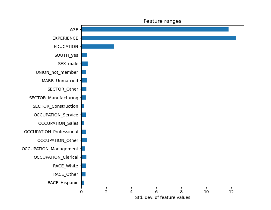
查看系数图来衡量特征重要性可能会产生误导,因为其中一些特征在小范围内变化,而另一些特征(如年龄 AGE)变化范围大得多,甚至长达数十年。
如果我们比较不同特征的标准差,这一点就很明显。
X_train_preprocessed = pd.DataFrame(
    model[:-1].transform(X_train), columns=feature_names
)

X_train_preprocessed.std(axis=0).plot.barh(figsize=(9, 7))
plt.title("Feature ranges")
plt.xlabel("Std. dev. of feature values")
plt.subplots_adjust(left=0.3)
将系数乘以相关特征的标准差将使所有系数统一到相同的计量单位。正如我们稍后将看到的,这等同于将数值变量归一化到其标准差,即 \(y = \sum{coef_i \times X_i} = \sum{(coef_i \times std_i) \times (X_i / std_i)}\)。
通过这种方式,我们强调,在其他条件不变的情况下,特征的方差越大,相应系数对输出的影响(权重)也越大。
coefs = pd.DataFrame(
    model[-1].regressor_.coef_ * X_train_preprocessed.std(axis=0),
    columns=["Coefficient importance"],
    index=feature_names,
)
coefs.plot(kind="barh", figsize=(9, 7))
plt.xlabel("Coefficient values corrected by the feature's std. dev.")
plt.title("Ridge model, small regularization")
plt.axvline(x=0, color=".5")
plt.subplots_adjust(left=0.3)
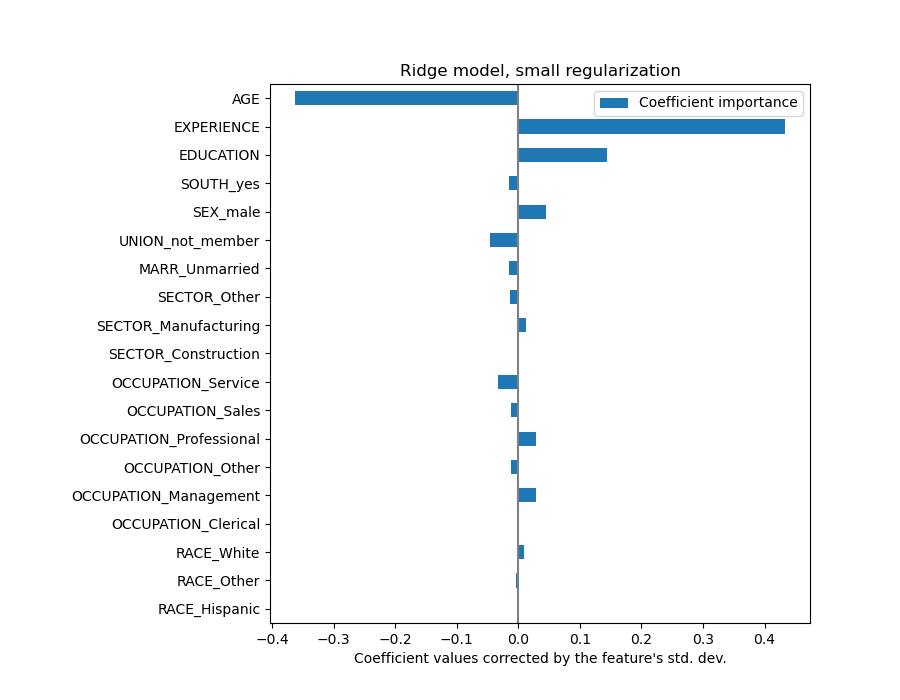
现在系数已经过缩放,我们可以安全地比较它们了。
警告
为什么上图显示年龄增长会导致工资下降?为什么初始配对图却显示相反的情况?
上图告诉我们,当所有其他特征保持不变时,特定特征与目标之间的依赖关系,即条件依赖性。当所有其他特征保持不变时,年龄(AGE)的增加将导致工资(WAGE)的减少。相反,当所有其他特征保持不变时,经验(EXPERIENCE)的增加将导致工资(WAGE)的增加。此外,年龄(AGE)、经验(EXPERIENCE)和教育(EDUCATION)是影响模型最大的三个变量。
解释系数:谨慎对待因果关系#
线性模型是衡量统计关联性的强大工具,但我们在谈论因果关系时应谨慎,毕竟相关性并不总是意味着因果关系。这在社会科学中尤其困难,因为我们观察到的变量只作为潜在因果过程的代理。
在我们的特定案例中,我们可以将个人的教育(EDUCATION)视为其职业能力(我们真正感兴趣但无法观察到的变量)的代理。我们当然希望在学校待得更久会提高技术能力,但因果关系也很有可能反过来。也就是说,那些技术能力强的人往往会在学校待更长时间。
雇主不太可能关心是哪种情况(或者两者兼有),只要他们仍然相信受过更多教育的人更适合这份工作,他们就会乐意支付更高的工资。
这种效应混杂在考虑某种形式的干预时会变得有问题,例如政府对大学学位的补贴或鼓励个人接受高等教育的宣传材料。这些措施的有效性最终可能会被夸大,尤其是当混杂程度很高时。我们的模型预测,每增加一年教育,每小时工资会增加 \(0.054699\)。由于这种混杂,实际的因果效应可能会更低。
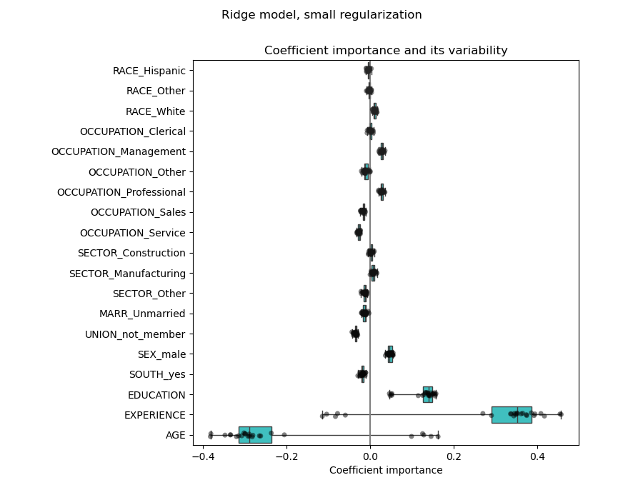
检查系数的变异性#
我们可以通过交叉验证检查系数的变异性:这是一种数据扰动形式(与重采样相关)。
如果系数在更改输入数据集时显著变化,则其鲁棒性无法保证,因此应谨慎解释。
from sklearn.model_selection import RepeatedKFold, cross_validate

cv = RepeatedKFold(n_splits=5, n_repeats=5, random_state=0)
cv_model = cross_validate(
    model,
    X,
    y,
    cv=cv,
    return_estimator=True,
    n_jobs=2,
)

coefs = pd.DataFrame(
    [
        est[-1].regressor_.coef_ * est[:-1].transform(X.iloc[train_idx]).std(axis=0)
        for est, (train_idx, _) in zip(cv_model["estimator"], cv.split(X, y))
    ],
    columns=feature_names,
)
plt.figure(figsize=(9, 7))
sns.stripplot(data=coefs, orient="h", palette="dark:k", alpha=0.5)
sns.boxplot(data=coefs, orient="h", color="cyan", saturation=0.5, whis=10)
plt.axvline(x=0, color=".5")
plt.xlabel("Coefficient importance")
plt.title("Coefficient importance and its variability")
plt.suptitle("Ridge model, small regularization")
plt.subplots_adjust(left=0.3)
相关变量的问题#
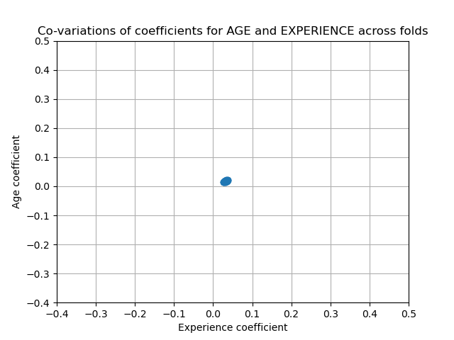
年龄(AGE)和经验(EXPERIENCE)系数受到强变异性的影响,这可能是由于这两个特征之间的共线性:随着年龄和经验在数据中一起变化,它们的影响难以区分。
为了验证这种解释,我们绘制了年龄(AGE)和经验(EXPERIENCE)系数的变异性。
plt.ylabel("Age coefficient")
plt.xlabel("Experience coefficient")
plt.grid(True)
plt.xlim(-0.4, 0.5)
plt.ylim(-0.4, 0.5)
plt.scatter(coefs["AGE"], coefs["EXPERIENCE"])
_ = plt.title("Co-variations of coefficients for AGE and EXPERIENCE across folds")
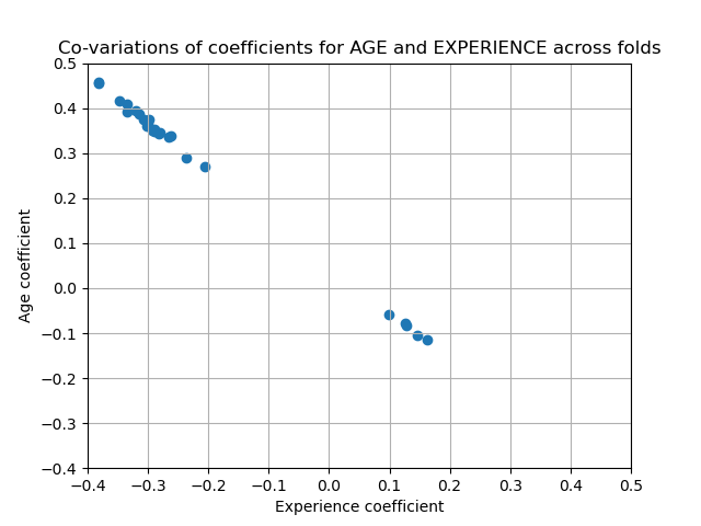
填充了两个区域:当经验系数为正时,年龄系数为负,反之亦然。
为了进一步探讨,我们删除其中一个特征,并检查它对模型稳定性的影响。
column_to_drop = ["AGE"]

cv_model = cross_validate(
    model,
    X.drop(columns=column_to_drop),
    y,
    cv=cv,
    return_estimator=True,
    n_jobs=2,
)

coefs = pd.DataFrame(
    [
        est[-1].regressor_.coef_
        * est[:-1].transform(X.drop(columns=column_to_drop).iloc[train_idx]).std(axis=0)
        for est, (train_idx, _) in zip(cv_model["estimator"], cv.split(X, y))
    ],
    columns=feature_names[:-1],
)
plt.figure(figsize=(9, 7))
sns.stripplot(data=coefs, orient="h", palette="dark:k", alpha=0.5)
sns.boxplot(data=coefs, orient="h", color="cyan", saturation=0.5)
plt.axvline(x=0, color=".5")
plt.title("Coefficient importance and its variability")
plt.xlabel("Coefficient importance")
plt.suptitle("Ridge model, small regularization, AGE dropped")
plt.subplots_adjust(left=0.3)
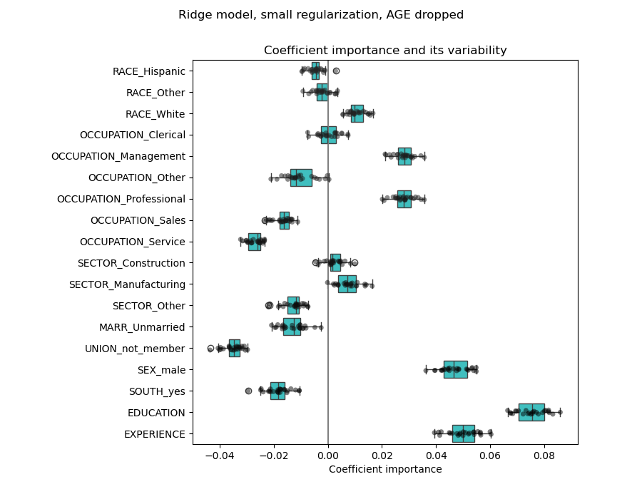
经验(EXPERIENCE)系数的估计现在显示出大大降低的变异性。在交叉验证期间训练的所有模型中,经验(EXPERIENCE)仍然很重要。
数值变量预处理#
如上所述(参见“机器学习流水线”),我们也可以选择在训练模型之前缩放数值。当我们对岭回归中的所有变量应用相似程度的正则化时,这可能很有用。预处理器被重新定义,以便减去均值并将变量缩放为单位方差。
from sklearn.preprocessing import StandardScaler

preprocessor = make_column_transformer(
    (OneHotEncoder(drop="if_binary"), categorical_columns),
    (StandardScaler(), numerical_columns),
)
模型将保持不变。
model = make_pipeline(
    preprocessor,
    TransformedTargetRegressor(
        regressor=Ridge(alpha=1e-10), func=np.log10, inverse_func=sp.special.exp10
    ),
)
model.fit(X_train, y_train)
再次,我们通过例如模型的中间绝对误差和 R 平方系数来检查计算模型的性能。
mae_train = median_absolute_error(y_train, model.predict(X_train))
y_pred = model.predict(X_test)
mae_test = median_absolute_error(y_test, y_pred)
scores = {
    "MedAE on training set": f"{mae_train:.2f} $/hour",
    "MedAE on testing set": f"{mae_test:.2f} $/hour",
}

_, ax = plt.subplots(figsize=(5, 5))
display = PredictionErrorDisplay.from_predictions(
    y_test, y_pred, kind="actual_vs_predicted", ax=ax, scatter_kwargs={"alpha": 0.5}
)
ax.set_title("Ridge model, small regularization")
for name, score in scores.items():
    ax.plot([], [], " ", label=f"{name}: {score}")
ax.legend(loc="upper left")
plt.tight_layout()
对于系数分析,这次不需要缩放,因为它已在预处理步骤中完成。
coefs = pd.DataFrame(
    model[-1].regressor_.coef_,
    columns=["Coefficients importance"],
    index=feature_names,
)
coefs.plot.barh(figsize=(9, 7))
plt.title("Ridge model, small regularization, normalized variables")
plt.xlabel("Raw coefficient values")
plt.axvline(x=0, color=".5")
plt.subplots_adjust(left=0.3)
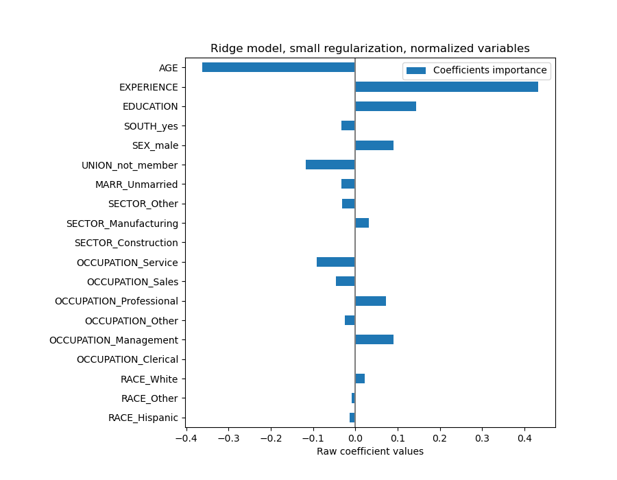
我们现在检查多个交叉验证折叠中的系数。与上面的示例一样,我们不需要根据特征值的标准差来缩放系数,因为此缩放已在流水线的预处理步骤中完成。
cv_model = cross_validate(
    model,
    X,
    y,
    cv=cv,
    return_estimator=True,
    n_jobs=2,
)
coefs = pd.DataFrame(
    [est[-1].regressor_.coef_ for est in cv_model["estimator"]], columns=feature_names
)
plt.figure(figsize=(9, 7))
sns.stripplot(data=coefs, orient="h", palette="dark:k", alpha=0.5)
sns.boxplot(data=coefs, orient="h", color="cyan", saturation=0.5, whis=10)
plt.axvline(x=0, color=".5")
plt.title("Coefficient variability")
plt.subplots_adjust(left=0.3)
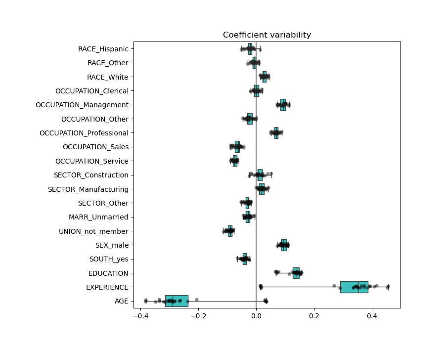
结果与未归一化的情况非常相似。
带有正则化的线性模型#
在机器学习实践中,岭回归通常与不可忽略的正则化一起使用。
上面,我们将这种正则化限制在非常小的量。正则化改善了问题的条件数并降低了估计的方差。RidgeCV 应用交叉验证以确定哪个正则化参数(alpha)值最适合预测。
from sklearn.linear_model import RidgeCV

alphas = np.logspace(-10, 10, 21)  # alpha values to be chosen from by cross-validation
model = make_pipeline(
    preprocessor,
    TransformedTargetRegressor(
        regressor=RidgeCV(alphas=alphas),
        func=np.log10,
        inverse_func=sp.special.exp10,
    ),
)
model.fit(X_train, y_train)
Pipeline(steps=[('columntransformer',
                 ColumnTransformer(transformers=[('onehotencoder',
                                                  OneHotEncoder(drop='if_binary'),
                                                  ['RACE', 'OCCUPATION',
                                                   'SECTOR', 'MARR', 'UNION',
                                                   'SEX', 'SOUTH']),
                                                 ('standardscaler',
                                                  StandardScaler(),
                                                  ['EDUCATION', 'EXPERIENCE',
                                                   'AGE'])])),
                ('transformedtargetregressor',
                 TransformedTargetRegressor(func=<ufunc 'log10'>,
                                            inverse_func=<ufunc 'exp10'>,
                                            regressor=RidgeCV(alphas=array([1.e-10, 1.e-09, 1.e-08, 1.e-07, 1.e-06, 1.e-05, 1.e-04, 1.e-03,
       1.e-02, 1.e-01, 1.e+00, 1.e+01, 1.e+02, 1.e+03, 1.e+04, 1.e+05,
       1.e+06, 1.e+07, 1.e+08, 1.e+09, 1.e+10]))))])
首先我们检查选择了哪个 \(\alpha\) 值。
model[-1].regressor_.alpha_
np.float64(10.0)
然后我们检查预测的质量。
mae_train = median_absolute_error(y_train, model.predict(X_train))
y_pred = model.predict(X_test)
mae_test = median_absolute_error(y_test, y_pred)
scores = {
    "MedAE on training set": f"{mae_train:.2f} $/hour",
    "MedAE on testing set": f"{mae_test:.2f} $/hour",
}

_, ax = plt.subplots(figsize=(5, 5))
display = PredictionErrorDisplay.from_predictions(
    y_test, y_pred, kind="actual_vs_predicted", ax=ax, scatter_kwargs={"alpha": 0.5}
)
ax.set_title("Ridge model, optimum regularization")
for name, score in scores.items():
    ax.plot([], [], " ", label=f"{name}: {score}")
ax.legend(loc="upper left")
plt.tight_layout()
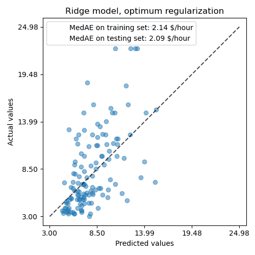
正则化模型重现数据的能力与非正则化模型相似。
coefs = pd.DataFrame(
    model[-1].regressor_.coef_,
    columns=["Coefficients importance"],
    index=feature_names,
)
coefs.plot.barh(figsize=(9, 7))
plt.title("Ridge model, with regularization, normalized variables")
plt.xlabel("Raw coefficient values")
plt.axvline(x=0, color=".5")
plt.subplots_adjust(left=0.3)
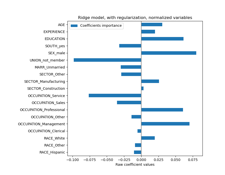
系数显著不同。年龄(AGE)和经验(EXPERIENCE)系数都是正的,但它们现在对预测的影响较小。
正则化降低了相关变量对模型的影响,因为权重在两个预测变量之间共享,因此任何一个单独的变量都不会有很大的权重。
另一方面,通过正则化获得的权重更稳定(参见 岭回归和分类 用户指南部分)。这种增加的稳定性可以从交叉验证中数据扰动得到的图中看出。这张图可以与前一张图进行比较。
cv_model = cross_validate(
    model,
    X,
    y,
    cv=cv,
    return_estimator=True,
    n_jobs=2,
)
coefs = pd.DataFrame(
    [est[-1].regressor_.coef_ for est in cv_model["estimator"]], columns=feature_names
)
plt.ylabel("Age coefficient")
plt.xlabel("Experience coefficient")
plt.grid(True)
plt.xlim(-0.4, 0.5)
plt.ylim(-0.4, 0.5)
plt.scatter(coefs["AGE"], coefs["EXPERIENCE"])
_ = plt.title("Co-variations of coefficients for AGE and EXPERIENCE across folds")
带有稀疏系数的线性模型#
另一种考虑数据集中相关变量的可能性是估计稀疏系数。在某种程度上,我们之前在岭回归估计中手动删除了年龄(AGE)列时已经做到了这一点。
Lasso 模型(参见 Lasso 用户指南部分)估计稀疏系数。LassoCV 应用交叉验证以确定哪个正则化参数(alpha)值最适合模型估计。
from sklearn.linear_model import LassoCV

alphas = np.logspace(-10, 10, 21)  # alpha values to be chosen from by cross-validation
model = make_pipeline(
    preprocessor,
    TransformedTargetRegressor(
        regressor=LassoCV(alphas=alphas, max_iter=100_000),
        func=np.log10,
        inverse_func=sp.special.exp10,
    ),
)

_ = model.fit(X_train, y_train)
首先我们验证选择了哪个 \(\alpha\) 值。
model[-1].regressor_.alpha_
np.float64(0.001)
然后我们检查预测的质量。
mae_train = median_absolute_error(y_train, model.predict(X_train))
y_pred = model.predict(X_test)
mae_test = median_absolute_error(y_test, y_pred)
scores = {
    "MedAE on training set": f"{mae_train:.2f} $/hour",
    "MedAE on testing set": f"{mae_test:.2f} $/hour",
}

_, ax = plt.subplots(figsize=(6, 6))
display = PredictionErrorDisplay.from_predictions(
    y_test, y_pred, kind="actual_vs_predicted", ax=ax, scatter_kwargs={"alpha": 0.5}
)
ax.set_title("Lasso model, optimum regularization")
for name, score in scores.items():
    ax.plot([], [], " ", label=f"{name}: {score}")
ax.legend(loc="upper left")
plt.tight_layout()
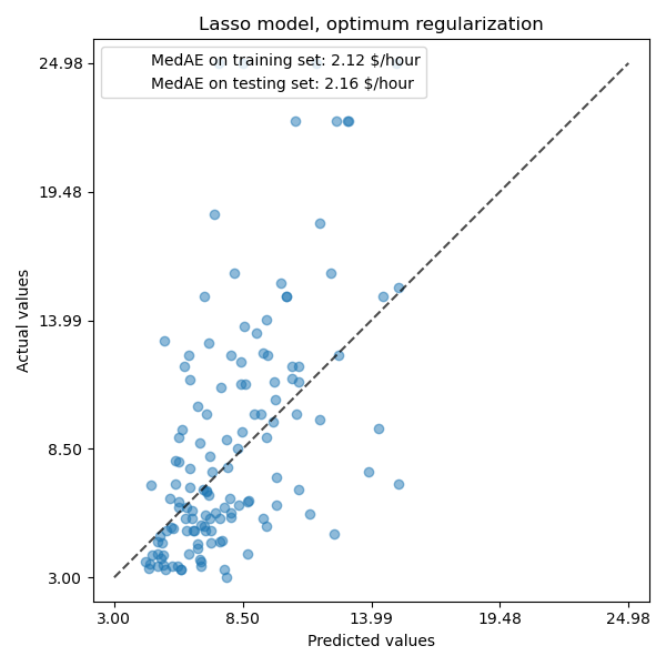
对于我们的数据集,该模型的预测能力仍然不强。
coefs = pd.DataFrame(
    model[-1].regressor_.coef_,
    columns=["Coefficients importance"],
    index=feature_names,
)
coefs.plot(kind="barh", figsize=(9, 7))
plt.title("Lasso model, optimum regularization, normalized variables")
plt.axvline(x=0, color=".5")
plt.subplots_adjust(left=0.3)
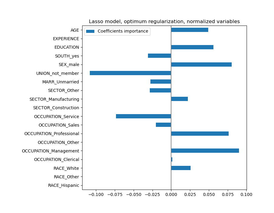
Lasso 模型识别年龄(AGE)和经验(EXPERIENCE)之间的相关性,并为了预测而抑制其中一个。
重要的是要记住,被丢弃的系数本身可能仍然与结果相关:模型选择抑制它们是因为它们在其他特征之上带来的额外信息很少或没有。此外,这种选择对于相关特征是不稳定的,应谨慎解释。
事实上,我们可以检查跨折叠的系数变异性。
cv_model = cross_validate(
    model,
    X,
    y,
    cv=cv,
    return_estimator=True,
    n_jobs=2,
)
coefs = pd.DataFrame(
    [est[-1].regressor_.coef_ for est in cv_model["estimator"]], columns=feature_names
)
plt.figure(figsize=(9, 7))
sns.stripplot(data=coefs, orient="h", palette="dark:k", alpha=0.5)
sns.boxplot(data=coefs, orient="h", color="cyan", saturation=0.5, whis=100)
plt.axvline(x=0, color=".5")
plt.title("Coefficient variability")
plt.subplots_adjust(left=0.3)
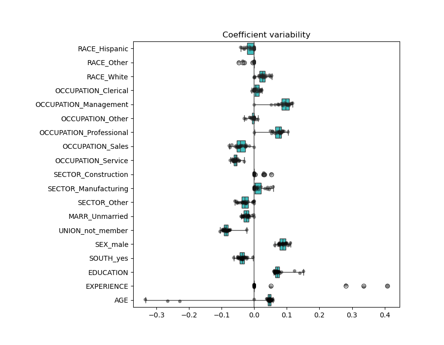
我们观察到年龄(AGE)和经验(EXPERIENCE)系数根据折叠(fold)的不同而变化很大。
错误的因果解释#
政策制定者可能希望了解教育对工资的影响,以评估旨在吸引人们接受更多教育的某项政策是否具有经济意义。虽然机器学习模型非常擅长衡量统计关联性,但它们通常无法推断因果效应。
看着我们最后一个模型(或任何模型)中教育对工资的系数,并得出结论认为它捕获了标准化教育变量变化对工资的真实影响,这可能很有诱惑力。
不幸的是,可能存在未观测到的混杂变量,它们会夸大或缩小该系数。混杂变量是指同时导致教育(EDUCATION)和工资(WAGE)的变量。这种变量的一个例子是能力。据推测,能力更强的人更有可能接受教育,同时在任何教育水平下也更有可能获得更高的时薪。在这种情况下,能力对教育系数产生了正的遗漏变量偏差(OVB),从而夸大了教育对工资的影响。
有关能力遗漏变量偏差 (OVB) 的模拟案例,请参阅机器学习无法推断因果效应。
经验教训#
系数必须缩放到相同的计量单位才能获取特征重要性。使用特征的标准差对其进行缩放是一个有用的代理。
当存在混杂效应时,解释因果关系是很困难的。如果两个变量之间的关系也受到某些未观测因素的影响,那么在得出因果关系结论时我们应该小心。
多元线性模型中的系数表示给定特征与目标之间的依赖关系,该依赖关系是以其他特征为条件的。
相关特征会导致线性模型系数的不稳定性,并且它们的影响无法很好地分离。
不同的线性模型对特征相关性的响应不同,并且系数之间可能显著不同。
检查交叉验证循环中各折叠的系数可以了解它们的稳定性。
系数不太可能具有任何因果意义。它们往往会受到未观测混杂因素的偏倚。
检查工具不一定能提供对真实数据生成过程的见解。
脚本总运行时间: (0 分钟 12.594 秒)
相关示例