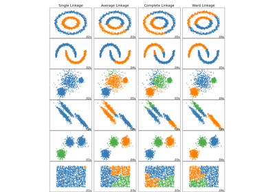
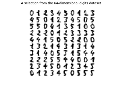
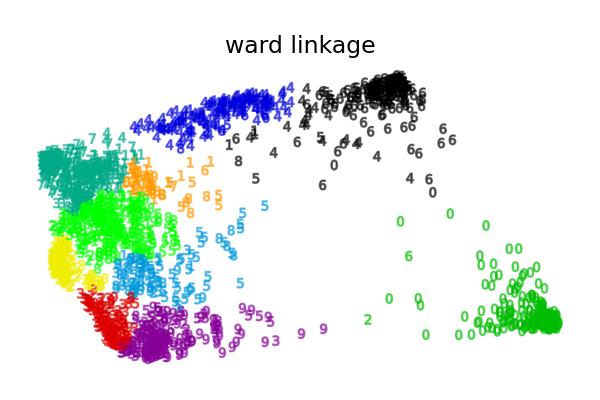
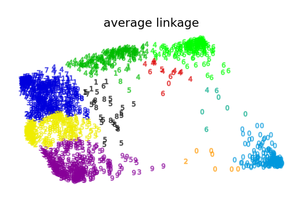
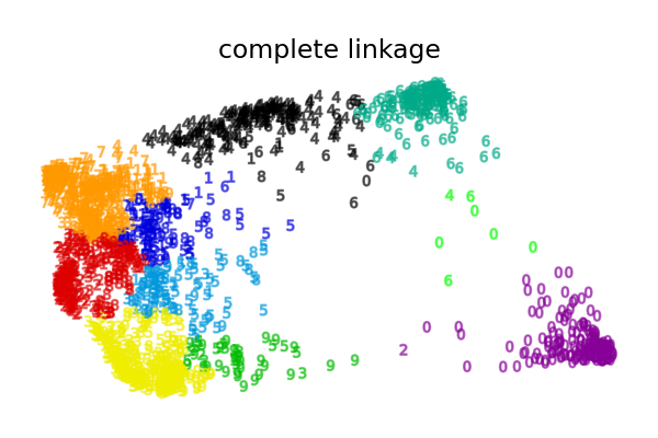
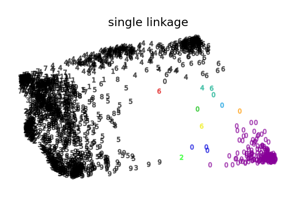
数字的二维嵌入上的各种聚合聚类#

这是对数字数据集的二维嵌入上，聚合聚类各种链接选项的说明。

此示例的目标是直观地展示这些度量的行为，而不是为数字找到好的聚类。这就是为什么此示例在二维嵌入上工作的原因。

此示例向我们展示了聚合聚类中“强者愈强”的行为，它倾向于创建不均匀的聚类大小。

这种行为在平均链接策略中尤为明显，该策略最终会形成几个数据点很少的聚类。

单链接的情况甚至更加病态，它会形成一个覆盖大多数数字的非常大的聚类，一个包含大多数零数字的中间大小（干净）聚类，而所有其他聚类则来自边缘附近的噪声点。

其他链接策略会产生更均匀分布的聚类，因此对数据集的随机重采样可能不那么敏感。

Computing embedding
Done.
ward :  0.05s
average :       0.05s
complete :      0.05s
single :        0.02s

# Authors: The scikit-learn developers
# SPDX-License-Identifier: BSD-3-Clause

from time import time

import numpy as np
from matplotlib import pyplot as plt

from sklearn import datasets, manifold

digits = datasets.load_digits()
X, y = digits.data, digits.target
n_samples, n_features = X.shape

np.random.seed(0)


# ----------------------------------------------------------------------
# Visualize the clustering
def plot_clustering(X_red, labels, title=None):
    x_min, x_max = np.min(X_red, axis=0), np.max(X_red, axis=0)
    X_red = (X_red - x_min) / (x_max - x_min)

    plt.figure(figsize=(6, 4))
    for digit in digits.target_names:
        plt.scatter(
            *X_red[y == digit].T,
            marker=f"${digit}$",
            s=50,
            c=plt.cm.nipy_spectral(labels[y == digit] / 10),
            alpha=0.5,
        )

    plt.xticks([])
    plt.yticks([])
    if title is not None:
        plt.title(title, size=17)
    plt.axis("off")
    plt.tight_layout(rect=[0, 0.03, 1, 0.95])


# ----------------------------------------------------------------------
# 2D embedding of the digits dataset
print("Computing embedding")
X_red = manifold.SpectralEmbedding(n_components=2).fit_transform(X)
print("Done.")

from sklearn.cluster import AgglomerativeClustering

for linkage in ("ward", "average", "complete", "single"):
    clustering = AgglomerativeClustering(linkage=linkage, n_clusters=10)
    t0 = time()
    clustering.fit(X_red)
    print("%s :\t%.2fs" % (linkage, time() - t0))

    plot_clustering(X_red, clustering.labels_, "%s linkage" % linkage)


plt.show()

脚本总运行时间： (0 分钟 1.402 秒)

数字的二维嵌入上的各种聚合聚类#

此页面