注
转到末尾 下载完整示例代码。或者通过 JupyterLite 或 Binder 在浏览器中运行此示例。
树集成特征变换#
将特征转换为高维稀疏空间。然后,在此特征上训练一个线性模型。
首先在训练集上拟合树集成(完全随机树、随机森林或梯度提升树)。然后,集成中每棵树的每个叶子都在新的特征空间中被分配一个固定的任意特征索引。这些叶子索引随后以独热(one-hot)方式编码。
每个样本都会经过集成中每棵树的决策,最终落在每棵树的一个叶子中。通过将这些叶子的特征值设为 1,其他特征值设为 0 来对样本进行编码。
得到的转换器学习了数据的有监督、稀疏、高维的类别嵌入。
# Authors: The scikit-learn developers
# SPDX-License-Identifier: BSD-3-Clause
首先,我们将创建一个大型数据集并将其分成三部分
用于训练集成方法的一个集合,这些方法随后用作特征工程转换器;
用于训练线性模型的一个集合;
用于测试线性模型的一个集合。
重要的是以这种方式划分数据,以避免因数据泄露而导致的过拟合。
from sklearn.datasets import make_classification
from sklearn.model_selection import train_test_split

X, y = make_classification(n_samples=80_000, random_state=10)

X_full_train, X_test, y_full_train, y_test = train_test_split(
    X, y, test_size=0.5, random_state=10
)
X_train_ensemble, X_train_linear, y_train_ensemble, y_train_linear = train_test_split(
    X_full_train, y_full_train, test_size=0.5, random_state=10
)
对于每种集成方法,我们将使用 10 个估计器和最大深度为 3 级。
n_estimators = 10
max_depth = 3
首先,我们将在分离的训练集上训练随机森林和梯度提升。
from sklearn.ensemble import GradientBoostingClassifier, RandomForestClassifier

random_forest = RandomForestClassifier(
    n_estimators=n_estimators, max_depth=max_depth, random_state=10
)
random_forest.fit(X_train_ensemble, y_train_ensemble)

gradient_boosting = GradientBoostingClassifier(
    n_estimators=n_estimators, max_depth=max_depth, random_state=10
)
_ = gradient_boosting.fit(X_train_ensemble, y_train_ensemble)
请注意,HistGradientBoostingClassifier 在中等规模数据集(n_samples >= 10_000)上比 GradientBoostingClassifier 快得多,但本示例不属于这种情况。
而 RandomTreesEmbedding 是一种无监督方法,因此不需要独立训练。
from sklearn.ensemble import RandomTreesEmbedding

random_tree_embedding = RandomTreesEmbedding(
    n_estimators=n_estimators, max_depth=max_depth, random_state=0
)
现在,我们将创建三个流水线,它们将使用上述嵌入作为预处理阶段。
随机树嵌入可以直接与逻辑回归通过流水线连接,因为它是一个标准的 scikit-learn 转换器。
from sklearn.linear_model import LogisticRegression
from sklearn.pipeline import make_pipeline

rt_model = make_pipeline(random_tree_embedding, LogisticRegression(max_iter=1000))
rt_model.fit(X_train_linear, y_train_linear)
然后,我们可以将随机森林或梯度提升与逻辑回归通过流水线连接。但是,特征变换将通过调用 apply 方法发生。scikit-learn 中的流水线期望调用 transform。因此,我们将对 apply 的调用封装在 FunctionTransformer 中。
from sklearn.preprocessing import FunctionTransformer, OneHotEncoder


def rf_apply(X, model):
    return model.apply(X)


rf_leaves_yielder = FunctionTransformer(rf_apply, kw_args={"model": random_forest})

rf_model = make_pipeline(
    rf_leaves_yielder,
    OneHotEncoder(handle_unknown="ignore"),
    LogisticRegression(max_iter=1000),
)
rf_model.fit(X_train_linear, y_train_linear)
def gbdt_apply(X, model):
    return model.apply(X)[:, :, 0]


gbdt_leaves_yielder = FunctionTransformer(
    gbdt_apply, kw_args={"model": gradient_boosting}
)

gbdt_model = make_pipeline(
    gbdt_leaves_yielder,
    OneHotEncoder(handle_unknown="ignore"),
    LogisticRegression(max_iter=1000),
)
gbdt_model.fit(X_train_linear, y_train_linear)
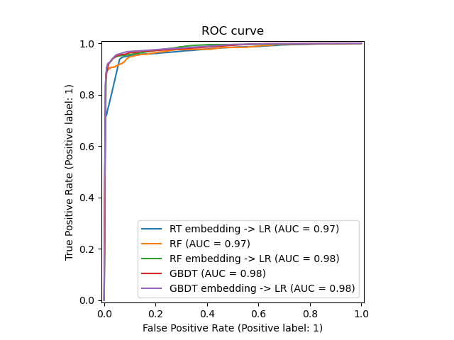
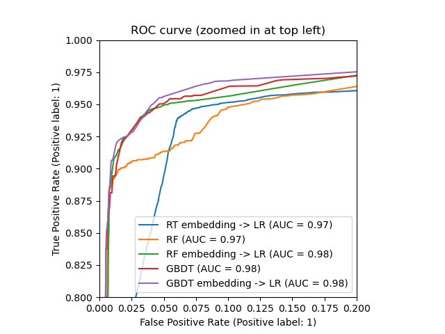
最后,我们可以展示所有模型的不同 ROC 曲线。
import matplotlib.pyplot as plt

from sklearn.metrics import RocCurveDisplay

_, ax = plt.subplots()

models = [
    ("RT embedding -> LR", rt_model),
    ("RF", random_forest),
    ("RF embedding -> LR", rf_model),
    ("GBDT", gradient_boosting),
    ("GBDT embedding -> LR", gbdt_model),
]

model_displays = {}
for name, pipeline in models:
    model_displays[name] = RocCurveDisplay.from_estimator(
        pipeline, X_test, y_test, ax=ax, name=name
    )
_ = ax.set_title("ROC curve")
_, ax = plt.subplots()
for name, pipeline in models:
    model_displays[name].plot(ax=ax)

ax.set_xlim(0, 0.2)
ax.set_ylim(0.8, 1)
_ = ax.set_title("ROC curve (zoomed in at top left)")
脚本总运行时间: (0 分钟 2.661 秒)
相关示例