注意
转到末尾 下载完整的示例代码。或者通过 JupyterLite 或 Binder 在浏览器中运行此示例
直方图梯度提升树中的特征#
基于直方图的梯度提升 (HGBT) 模型可能是 scikit-learn 中最有用的监督学习模型之一。它们基于与 LightGBM 和 XGBoost 可比的现代梯度提升实现。因此,HGBT 模型比随机森林等替代模型具有更丰富的特征,并且通常性能更优,尤其是在样本数量超过数万时(参见比较随机森林和直方图梯度提升模型)。
HGBT 模型的主要可用性特征包括:
本示例旨在展示除第2点和第6点外的所有特性在实际场景中的应用。
# Authors: The scikit-learn developers
# SPDX-License-Identifier: BSD-3-Clause
准备数据#
电力数据集包含从澳大利亚新南威尔士州电力市场收集的数据。在这个市场中,价格并非固定不变,而是受供需关系影响。价格每五分钟设定一次。为了缓解波动,会进行新南威尔士州与邻近维多利亚州之间的电力传输。
该数据集最初名为 ELEC2,包含从 1996 年 5 月 7 日到 1998 年 12 月 5 日的 45,312 个实例。数据集中的每个样本代表 30 分钟的时间段,即一天中的每个时间段有 48 个实例。数据集中的每个样本有 7 列:
date:1996 年 5 月 7 日至 1998 年 12 月 5 日之间。归一化到 0 和 1 之间;
day:星期几 (1-7);
period:24 小时内的半小时间隔。归一化到 0 和 1 之间;
nswprice/nswdemand:新南威尔士州的电价/电力需求;
vicprice/vicdemand:维多利亚州的电价/电力需求。
最初这是一个分类任务,但在这里我们将其用于回归任务,以预测州际之间计划的电力传输。
from sklearn.datasets import fetch_openml

electricity = fetch_openml(
    name="electricity", version=1, as_frame=True, parser="pandas"
)
df = electricity.frame
这个特定数据集在前 17,760 个样本中有一个阶梯式常数目标。
df["transfer"][:17_760].unique()
array([0.414912, 0.500526])
让我们删除这些条目,并探索一周中不同日期的每小时电力传输情况。
import matplotlib.pyplot as plt
import seaborn as sns

df = electricity.frame.iloc[17_760:]
X = df.drop(columns=["transfer", "class"])
y = df["transfer"]

fig, ax = plt.subplots(figsize=(15, 10))
pointplot = sns.lineplot(x=df["period"], y=df["transfer"], hue=df["day"], ax=ax)
handles, labels = ax.get_legend_handles_labels()
ax.set(
    title="Hourly energy transfer for different days of the week",
    xlabel="Normalized time of the day",
    ylabel="Normalized energy transfer",
)
_ = ax.legend(handles, ["Sun", "Mon", "Tue", "Wed", "Thu", "Fri", "Sat"])
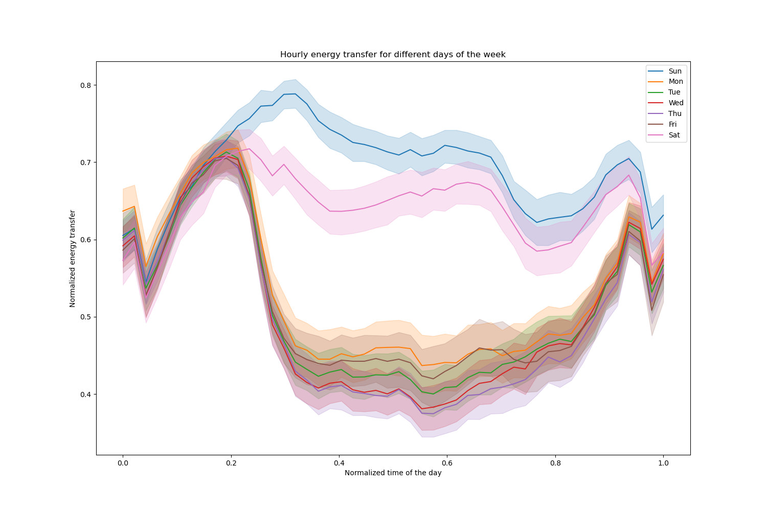
注意到周末期间能源传输系统性地增加。
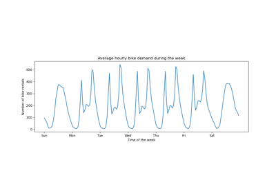
树的数量和早停的效果#
为了说明(最大)树数量的影响,我们使用整个数据集训练了一个HistGradientBoostingRegressor 来预测每日电力传输。然后我们根据 max_iter 参数可视化其预测。这里我们不尝试评估模型的性能及其泛化能力,而是评估其从训练数据中学习的能力。
from sklearn.ensemble import HistGradientBoostingRegressor
from sklearn.model_selection import train_test_split

X_train, X_test, y_train, y_test = train_test_split(X, y, test_size=0.4, shuffle=False)

print(f"Training sample size: {X_train.shape[0]}")
print(f"Test sample size: {X_test.shape[0]}")
print(f"Number of features: {X_train.shape[1]}")
Training sample size: 16531
Test sample size: 11021
Number of features: 7
max_iter_list = [5, 50]
average_week_demand = (
    df.loc[X_test.index].groupby(["day", "period"], observed=False)["transfer"].mean()
)
colors = sns.color_palette("colorblind")
fig, ax = plt.subplots(figsize=(10, 5))
average_week_demand.plot(color=colors[0], label="recorded average", linewidth=2, ax=ax)

for idx, max_iter in enumerate(max_iter_list):
    hgbt = HistGradientBoostingRegressor(
        max_iter=max_iter, categorical_features=None, random_state=42
    )
    hgbt.fit(X_train, y_train)

    y_pred = hgbt.predict(X_test)
    prediction_df = df.loc[X_test.index].copy()
    prediction_df["y_pred"] = y_pred
    average_pred = prediction_df.groupby(["day", "period"], observed=False)[
        "y_pred"
    ].mean()
    average_pred.plot(
        color=colors[idx + 1], label=f"max_iter={max_iter}", linewidth=2, ax=ax
    )

ax.set(
    title="Predicted average energy transfer during the week",
    xticks=[(i + 0.2) * 48 for i in range(7)],
    xticklabels=["Sun", "Mon", "Tue", "Wed", "Thu", "Fri", "Sat"],
    xlabel="Time of the week",
    ylabel="Normalized energy transfer",
)
_ = ax.legend()
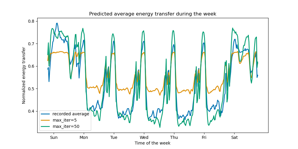
仅通过几次迭代,HGBT 模型就能达到收敛(参见比较随机森林和直方图梯度提升模型),这意味着添加更多树不再能改善模型。在上面的图中,5 次迭代不足以获得良好的预测。而 50 次迭代,我们已经能够做得很好。
将 max_iter 设置得过高可能会降低预测质量并浪费大量可避免的计算资源。因此,scikit-learn 中的 HGBT 实现提供了一种自动的早停策略。通过该策略,模型将一部分训练数据用作内部验证集(validation_fraction),并且如果在 n_iter_no_change 次迭代后验证分数没有改善(或下降),则停止训练,直到达到某个容差(tol)。
注意到 learning_rate 和 max_iter 之间存在权衡:一般来说,较小的学习率更受青睐,但需要更多迭代才能收敛到最小损失,而较大的学习率收敛更快(所需迭代/树更少),但代价是最小损失更大。
由于学习率和迭代次数之间的高度相关性,一个好的做法是,将学习率与其他所有(重要的)超参数一起调优,在训练集上使用足够大的 max_iter 值拟合 HBGT,并通过早停和一些显式的 validation_fraction 来确定最佳的 max_iter。
common_params = {
    "max_iter": 1_000,
    "learning_rate": 0.3,
    "validation_fraction": 0.2,
    "random_state": 42,
    "categorical_features": None,
    "scoring": "neg_root_mean_squared_error",
}

hgbt = HistGradientBoostingRegressor(early_stopping=True, **common_params)
hgbt.fit(X_train, y_train)

_, ax = plt.subplots()
plt.plot(-hgbt.validation_score_)
_ = ax.set(
    xlabel="number of iterations",
    ylabel="root mean squared error",
    title=f"Loss of hgbt with early stopping (n_iter={hgbt.n_iter_})",
)
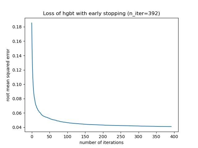
然后我们可以将 max_iter 的值覆盖为一个合理的值,从而避免内部验证的额外计算成本。将迭代次数向上取整可能可以应对训练集的变异性。
import math

common_params["max_iter"] = math.ceil(hgbt.n_iter_ / 100) * 100
common_params["early_stopping"] = False
hgbt = HistGradientBoostingRegressor(**common_params)
注意
早停期间进行的内部验证对于时间序列不是最优的。
缺失值支持#
HGBT 模型原生支持缺失值。在训练期间,树生长器会根据潜在增益,在每次分裂时决定缺失值样本应该去哪里(左子节点或右子节点)。预测时,这些样本会相应地发送到已学习的子节点。如果一个特征在训练期间没有缺失值,那么在预测时,该特征有缺失值的样本将被发送到样本最多的子节点(如在拟合期间所见)。
本示例展示了 HGBT 回归如何处理完全随机缺失 (MCAR) 的值,即缺失与观测数据或未观测数据无关。我们可以通过随机将选定特征中的值替换为 nan 值来模拟这种情况。
import numpy as np

from sklearn.metrics import root_mean_squared_error

rng = np.random.RandomState(42)
first_week = slice(0, 336)  # first week in the test set as 7 * 48 = 336
missing_fraction_list = [0, 0.01, 0.03]


def generate_missing_values(X, missing_fraction):
    total_cells = X.shape[0] * X.shape[1]
    num_missing_cells = int(total_cells * missing_fraction)
    row_indices = rng.choice(X.shape[0], num_missing_cells, replace=True)
    col_indices = rng.choice(X.shape[1], num_missing_cells, replace=True)
    X_missing = X.copy()
    X_missing.iloc[row_indices, col_indices] = np.nan
    return X_missing


fig, ax = plt.subplots(figsize=(12, 6))
ax.plot(y_test.values[first_week], label="Actual transfer")

for missing_fraction in missing_fraction_list:
    X_train_missing = generate_missing_values(X_train, missing_fraction)
    X_test_missing = generate_missing_values(X_test, missing_fraction)
    hgbt.fit(X_train_missing, y_train)
    y_pred = hgbt.predict(X_test_missing[first_week])
    rmse = root_mean_squared_error(y_test[first_week], y_pred)
    ax.plot(
        y_pred[first_week],
        label=f"missing_fraction={missing_fraction}, RMSE={rmse:.3f}",
        alpha=0.5,
    )
ax.set(
    title="Daily energy transfer predictions on data with MCAR values",
    xticks=[(i + 0.2) * 48 for i in range(7)],
    xticklabels=["Mon", "Tue", "Wed", "Thu", "Fri", "Sat", "Sun"],
    xlabel="Time of the week",
    ylabel="Normalized energy transfer",
)
_ = ax.legend(loc="lower right")
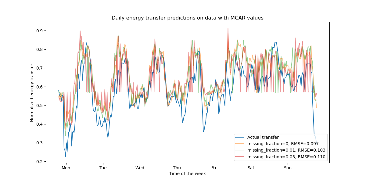
正如预期,随着缺失值比例的增加,模型性能会下降。
分位数损失支持#
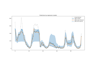
回归中的分位数损失能够展示目标变量的变异性或不确定性。例如,预测第 5 和第 95 百分位数可以提供 90% 的预测区间,即我们期望新观测值以 90% 概率落入的范围。
from sklearn.metrics import mean_pinball_loss

quantiles = [0.95, 0.05]
predictions = []

fig, ax = plt.subplots(figsize=(12, 6))
ax.plot(y_test.values[first_week], label="Actual transfer")

for quantile in quantiles:
    hgbt_quantile = HistGradientBoostingRegressor(
        loss="quantile", quantile=quantile, **common_params
    )
    hgbt_quantile.fit(X_train, y_train)
    y_pred = hgbt_quantile.predict(X_test[first_week])

    predictions.append(y_pred)
    score = mean_pinball_loss(y_test[first_week], y_pred)
    ax.plot(
        y_pred[first_week],
        label=f"quantile={quantile}, pinball loss={score:.2f}",
        alpha=0.5,
    )

ax.fill_between(
    range(len(predictions[0][first_week])),
    predictions[0][first_week],
    predictions[1][first_week],
    color=colors[0],
    alpha=0.1,
)
ax.set(
    title="Daily energy transfer predictions with quantile loss",
    xticks=[(i + 0.2) * 48 for i in range(7)],
    xticklabels=["Mon", "Tue", "Wed", "Thu", "Fri", "Sat", "Sun"],
    xlabel="Time of the week",
    ylabel="Normalized energy transfer",
)
_ = ax.legend(loc="lower right")
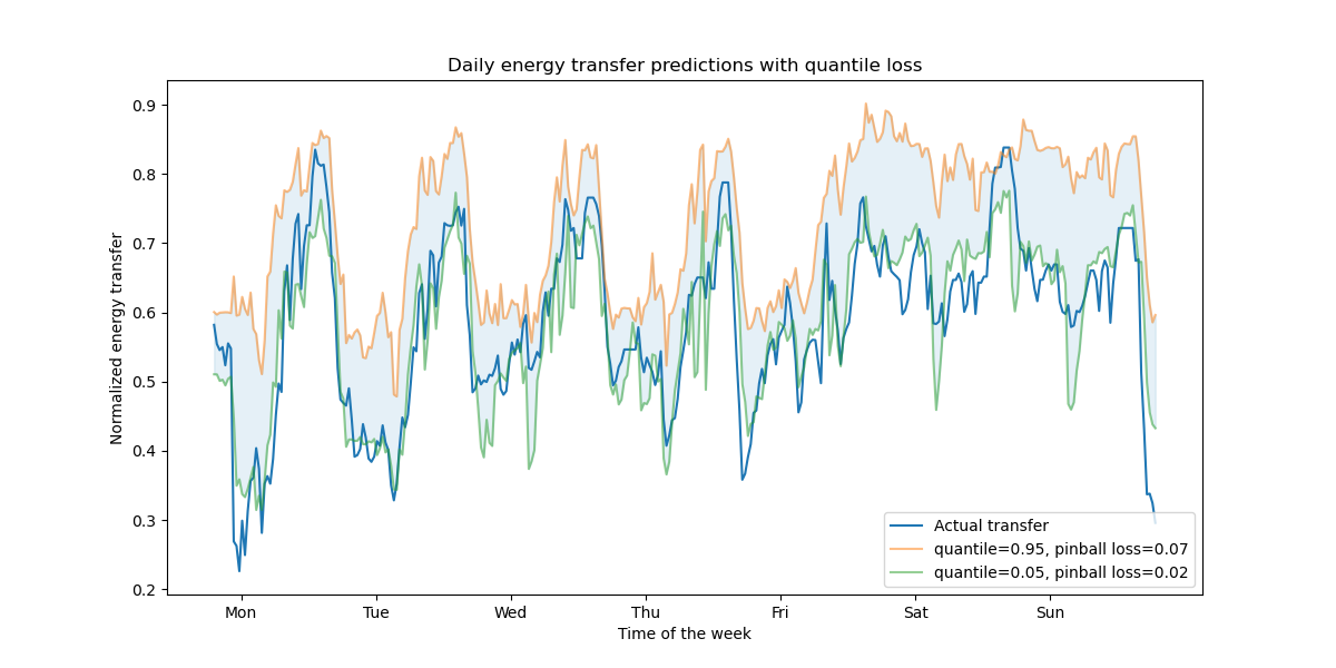
我们观察到能量传输有高估的趋势。这可以通过计算经验覆盖率来定量确认,如置信区间校准部分所示。请记住,这些预测的百分位数只是模型估计值。通过以下方式仍然可以提高这些估计的质量:
收集更多数据点;
更好地调优模型超参数,参见梯度提升回归的预测区间;
从相同数据中设计更多预测性特征,参见时间相关特征工程。
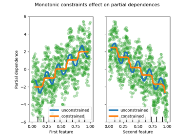
单调约束#
鉴于特定的领域知识要求特征与目标之间的关系是单调递增或递减的,可以使用单调约束在 HGBT 模型的预测中强制执行这种行为。这使得模型更具可解释性,并能降低其方差(并可能减轻过拟合),但有增加偏差的风险。单调约束还可以用于强制执行特定的监管要求,确保合规性并与伦理考虑相符。
在本示例中,将能源从维多利亚州转移到新南威尔士州的政策旨在缓解价格波动,这意味着模型预测必须强制执行这一目标,即转移量应随新南威尔士州的价格和需求增加而增加,但同时应随维多利亚州的价格和需求增加而减少,以使两地民众受益。
如果训练数据包含特征名称,可以通过传递一个遵循以下约定的字典来指定单调约束:
1: 单调递增
0: 无约束
-1: 单调递减
另外,也可以传递一个数组状对象,按位置编码上述约定。
from sklearn.inspection import PartialDependenceDisplay

monotonic_cst = {
    "date": 0,
    "day": 0,
    "period": 0,
    "nswdemand": 1,
    "nswprice": 1,
    "vicdemand": -1,
    "vicprice": -1,
}
hgbt_no_cst = HistGradientBoostingRegressor(
    categorical_features=None, random_state=42
).fit(X, y)
hgbt_cst = HistGradientBoostingRegressor(
    monotonic_cst=monotonic_cst, categorical_features=None, random_state=42
).fit(X, y)

fig, ax = plt.subplots(nrows=2, figsize=(15, 10))
disp = PartialDependenceDisplay.from_estimator(
    hgbt_no_cst,
    X,
    features=["nswdemand", "nswprice"],
    line_kw={"linewidth": 2, "label": "unconstrained", "color": "tab:blue"},
    ax=ax[0],
)
PartialDependenceDisplay.from_estimator(
    hgbt_cst,
    X,
    features=["nswdemand", "nswprice"],
    line_kw={"linewidth": 2, "label": "constrained", "color": "tab:orange"},
    ax=disp.axes_,
)
disp = PartialDependenceDisplay.from_estimator(
    hgbt_no_cst,
    X,
    features=["vicdemand", "vicprice"],
    line_kw={"linewidth": 2, "label": "unconstrained", "color": "tab:blue"},
    ax=ax[1],
)
PartialDependenceDisplay.from_estimator(
    hgbt_cst,
    X,
    features=["vicdemand", "vicprice"],
    line_kw={"linewidth": 2, "label": "constrained", "color": "tab:orange"},
    ax=disp.axes_,
)
_ = plt.legend()
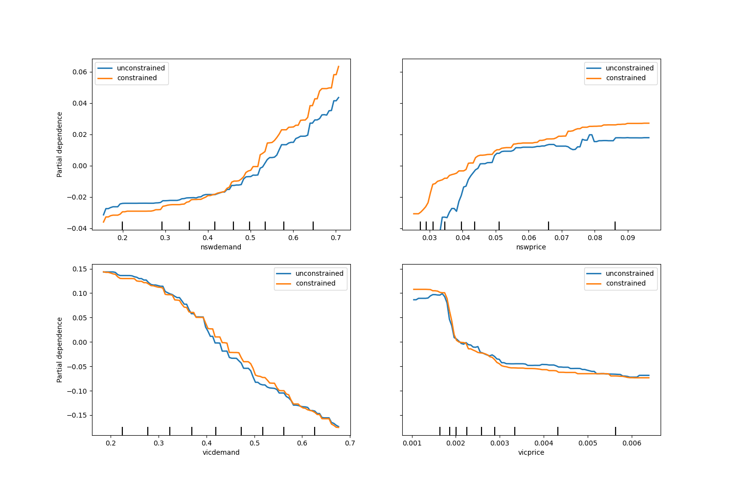
观察到 nswdemand 和 vicdemand 在没有约束的情况下似乎已经单调。这是一个很好的例子,说明带有单调性约束的模型是“过度约束”的。
此外,我们可以验证引入单调约束后,模型的预测质量没有显著下降。为此,我们使用TimeSeriesSplit 交叉验证来估计测试分数的方差。通过这样做,我们保证训练数据不会“看到”测试数据之后的数据,这在处理具有时间关系的数据时至关重要。
from sklearn.metrics import make_scorer, root_mean_squared_error
from sklearn.model_selection import TimeSeriesSplit, cross_validate

ts_cv = TimeSeriesSplit(n_splits=5, gap=48, test_size=336)  # a week has 336 samples
scorer = make_scorer(root_mean_squared_error)

cv_results = cross_validate(hgbt_no_cst, X, y, cv=ts_cv, scoring=scorer)
rmse = cv_results["test_score"]
print(f"RMSE without constraints = {rmse.mean():.3f} +/- {rmse.std():.3f}")

cv_results = cross_validate(hgbt_cst, X, y, cv=ts_cv, scoring=scorer)
rmse = cv_results["test_score"]
print(f"RMSE with constraints    = {rmse.mean():.3f} +/- {rmse.std():.3f}")
RMSE without constraints = 0.103 +/- 0.030
RMSE with constraints    = 0.107 +/- 0.034
话虽如此,请注意,此比较是在两个可能通过不同超参数组合进行优化的不同模型之间进行的。这就是为什么我们在此部分不像之前那样使用 common_params 的原因。
脚本总运行时间: (0 分钟 19.658 秒)
相关示例