回归模型中目标变量变换的效果

本示例概述了 TransformedTargetRegressor。我们使用两个示例来说明在学习线性回归模型之前对目标变量进行变换的好处。第一个示例使用合成数据，而第二个示例基于 Ames 住房数据集。

# Authors: The scikit-learn developers
# SPDX-License-Identifier: BSD-3-Clause

print(__doc__)

合成数据示例

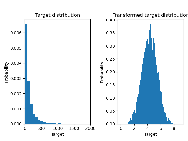
生成了一个合成的随机回归数据集。目标变量 y 通过以下方式进行修改：

1. 平移所有目标变量，使所有值非负（通过加上最低 y 的绝对值），以及

2. 应用指数函数以获得无法使用简单线性模型拟合的非线性目标变量。

因此，在训练线性回归模型并用于预测之前，将使用对数函数（np.log1p）和指数函数（np.expm1）来变换目标变量。

import numpy as np

from sklearn.datasets import make_regression

X, y = make_regression(n_samples=10_000, noise=100, random_state=0)
y = np.expm1((y + abs(y.min())) / 200)
y_trans = np.log1p(y)

下面我们绘制了应用对数函数前后目标变量的概率密度函数。

import matplotlib.pyplot as plt

from sklearn.model_selection import train_test_split

f, (ax0, ax1) = plt.subplots(1, 2)

ax0.hist(y, bins=100, density=True)
ax0.set_xlim([0, 2000])
ax0.set_ylabel("Probability")
ax0.set_xlabel("Target")
ax0.set_title("Target distribution")

ax1.hist(y_trans, bins=100, density=True)
ax1.set_ylabel("Probability")
ax1.set_xlabel("Target")
ax1.set_title("Transformed target distribution")

f.suptitle("Synthetic data", y=1.05)
plt.tight_layout()

X_train, X_test, y_train, y_test = train_test_split(X, y, random_state=0)

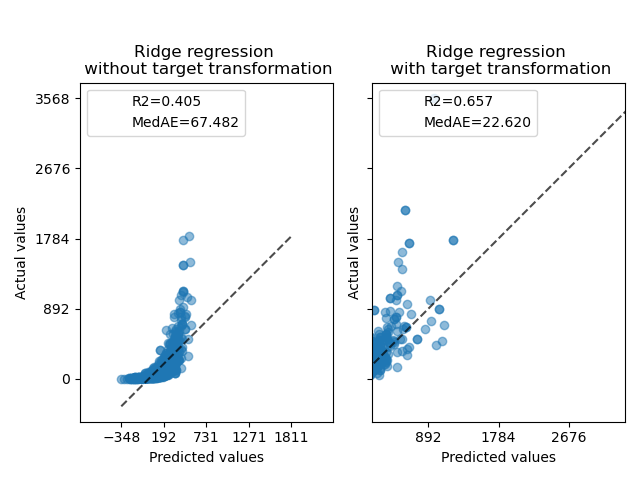
首先，将在线性模型应用于原始目标变量。由于非线性，训练出的模型在预测时不会很精确。随后，使用对数函数将目标变量线性化，即使使用类似的线性模型，也能获得更好的预测结果，如中位数绝对误差 (MedAE) 所示。

from sklearn.metrics import median_absolute_error, r2_score


def compute_score(y_true, y_pred):
    return {
        "R2": f"{r2_score(y_true, y_pred):.3f}",
        "MedAE": f"{median_absolute_error(y_true, y_pred):.3f}",
    }

from sklearn.compose import TransformedTargetRegressor
from sklearn.linear_model import RidgeCV
from sklearn.metrics import PredictionErrorDisplay

f, (ax0, ax1) = plt.subplots(1, 2, sharey=True)

ridge_cv = RidgeCV().fit(X_train, y_train)
y_pred_ridge = ridge_cv.predict(X_test)

ridge_cv_with_trans_target = TransformedTargetRegressor(
    regressor=RidgeCV(), func=np.log1p, inverse_func=np.expm1
).fit(X_train, y_train)
y_pred_ridge_with_trans_target = ridge_cv_with_trans_target.predict(X_test)

PredictionErrorDisplay.from_predictions(
    y_test,
    y_pred_ridge,
    kind="actual_vs_predicted",
    ax=ax0,
    scatter_kwargs={"alpha": 0.5},
)
PredictionErrorDisplay.from_predictions(
    y_test,
    y_pred_ridge_with_trans_target,
    kind="actual_vs_predicted",
    ax=ax1,
    scatter_kwargs={"alpha": 0.5},
)

# Add the score in the legend of each axis
for ax, y_pred in zip([ax0, ax1], [y_pred_ridge, y_pred_ridge_with_trans_target]):
    for name, score in compute_score(y_test, y_pred).items():
        ax.plot([], [], " ", label=f"{name}={score}")
    ax.legend(loc="upper left")

ax0.set_title("Ridge regression \n without target transformation")
ax1.set_title("Ridge regression \n with target transformation")
f.suptitle("Synthetic data", y=1.05)
plt.tight_layout()

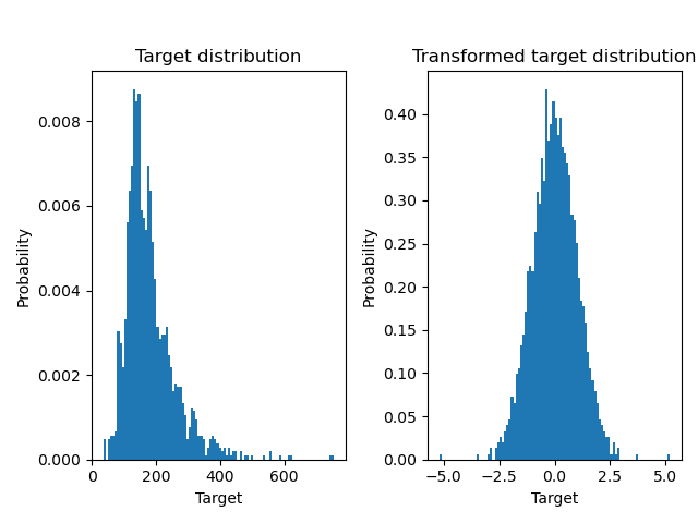
真实世界数据集

类似地，使用 Ames 住房数据集来展示在学习模型之前对目标变量进行变换的影响。在本示例中，要预测的目标是每套房屋的售价。

from sklearn.datasets import fetch_openml
from sklearn.preprocessing import quantile_transform

ames = fetch_openml(name="house_prices", as_frame=True)
# Keep only numeric columns
X = ames.data.select_dtypes(np.number)
# Remove columns with NaN or Inf values
X = X.drop(columns=["LotFrontage", "GarageYrBlt", "MasVnrArea"])
# Let the price be in k$
y = ames.target / 1000
y_trans = quantile_transform(
    y.to_frame(), n_quantiles=900, output_distribution="normal", copy=True
).squeeze()

在应用 RidgeCV 模型之前，使用 QuantileTransformer 来标准化目标变量分布。

f, (ax0, ax1) = plt.subplots(1, 2)

ax0.hist(y, bins=100, density=True)
ax0.set_ylabel("Probability")
ax0.set_xlabel("Target")
ax0.set_title("Target distribution")

ax1.hist(y_trans, bins=100, density=True)
ax1.set_ylabel("Probability")
ax1.set_xlabel("Target")
ax1.set_title("Transformed target distribution")

f.suptitle("Ames housing data: selling price", y=1.05)
plt.tight_layout()

X_train, X_test, y_train, y_test = train_test_split(X, y, random_state=1)

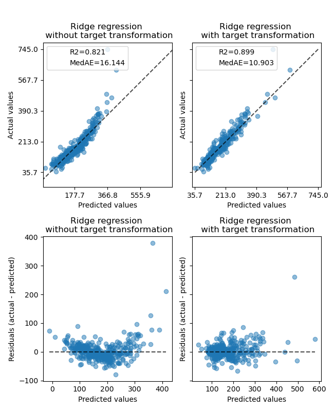
变换器的效果弱于合成数据。然而，变换导致 \(R^2\) 增加，并且 MedAE 大幅下降。在不进行目标变量变换的情况下，残差图（预测目标 - 真实目标 vs 预测目标）呈现出弯曲的“反向微笑”形状，这是因为残差值会随预测目标的值而变化。进行目标变量变换后，形状更趋于线性，表明模型拟合更好。

from sklearn.preprocessing import QuantileTransformer

f, (ax0, ax1) = plt.subplots(2, 2, sharey="row", figsize=(6.5, 8))

ridge_cv = RidgeCV().fit(X_train, y_train)
y_pred_ridge = ridge_cv.predict(X_test)

ridge_cv_with_trans_target = TransformedTargetRegressor(
    regressor=RidgeCV(),
    transformer=QuantileTransformer(n_quantiles=900, output_distribution="normal"),
).fit(X_train, y_train)
y_pred_ridge_with_trans_target = ridge_cv_with_trans_target.predict(X_test)

# plot the actual vs predicted values
PredictionErrorDisplay.from_predictions(
    y_test,
    y_pred_ridge,
    kind="actual_vs_predicted",
    ax=ax0[0],
    scatter_kwargs={"alpha": 0.5},
)
PredictionErrorDisplay.from_predictions(
    y_test,
    y_pred_ridge_with_trans_target,
    kind="actual_vs_predicted",
    ax=ax0[1],
    scatter_kwargs={"alpha": 0.5},
)

# Add the score in the legend of each axis
for ax, y_pred in zip([ax0[0], ax0[1]], [y_pred_ridge, y_pred_ridge_with_trans_target]):
    for name, score in compute_score(y_test, y_pred).items():
        ax.plot([], [], " ", label=f"{name}={score}")
    ax.legend(loc="upper left")

ax0[0].set_title("Ridge regression \n without target transformation")
ax0[1].set_title("Ridge regression \n with target transformation")

# plot the residuals vs the predicted values
PredictionErrorDisplay.from_predictions(
    y_test,
    y_pred_ridge,
    kind="residual_vs_predicted",
    ax=ax1[0],
    scatter_kwargs={"alpha": 0.5},
)
PredictionErrorDisplay.from_predictions(
    y_test,
    y_pred_ridge_with_trans_target,
    kind="residual_vs_predicted",
    ax=ax1[1],
    scatter_kwargs={"alpha": 0.5},
)
ax1[0].set_title("Ridge regression \n without target transformation")
ax1[1].set_title("Ridge regression \n with target transformation")

f.suptitle("Ames housing data: selling price", y=1.05)
plt.tight_layout()
plt.show()

相关示例

等渗回归

等渗回归

Pipeline：链式连接 PCA 和逻辑回归

Pipeline：链式连接 PCA 和逻辑回归

绘制交叉验证预测

绘制交叉验证预测

使用 stacking 组合预测器

使用 stacking 组合预测器