使用邻域成分分析进行降维#

邻域成分分析在降维中的示例用法。

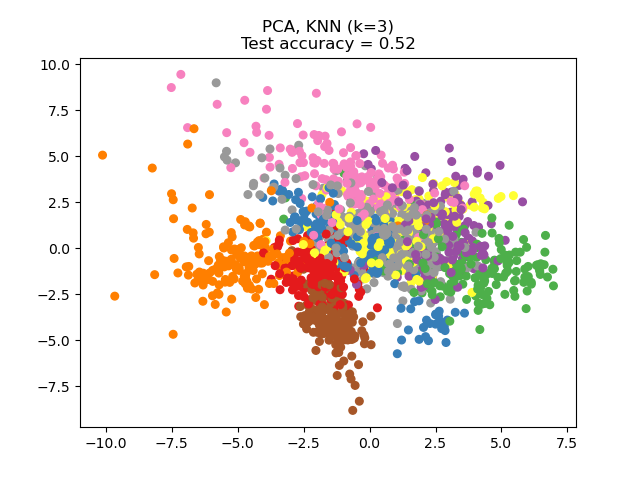
此示例比较了应用于数字数据集的不同（线性）降维方法。该数据集包含从 0 到 9 的数字图像，每个类别约有 180 个样本。每张图像的维度为 8x8 = 64，并被降维到二维数据点。

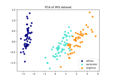
应用于此数据的主成分分析 (PCA) 识别出解释数据中最大方差的属性组合（主成分，或特征空间中的方向）。在此处，我们绘制了不同样本在最初的 2 个主成分上的分布。

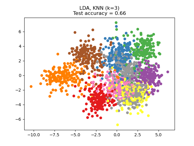
线性判别分析 (LDA) 试图识别解释最大方差的属性类别之间。特别是，与 PCA 相比，LDA 是一种监督方法，使用已知的类别标签。

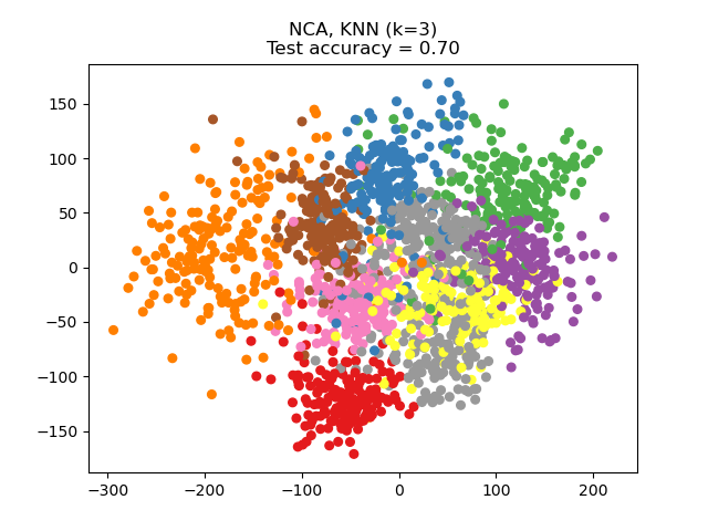
邻域成分分析 (NCA) 试图找到一个特征空间，使得随机最近邻算法能提供最佳准确度。与 LDA 类似，它是一种监督方法。

可以看出，尽管维度大幅降低，NCA 仍能实现数据聚类，且具有视觉意义。

# Authors: The scikit-learn developers
# SPDX-License-Identifier: BSD-3-Clause

import matplotlib.pyplot as plt
import numpy as np

from sklearn import datasets
from sklearn.decomposition import PCA
from sklearn.discriminant_analysis import LinearDiscriminantAnalysis
from sklearn.model_selection import train_test_split
from sklearn.neighbors import KNeighborsClassifier, NeighborhoodComponentsAnalysis
from sklearn.pipeline import make_pipeline
from sklearn.preprocessing import StandardScaler

n_neighbors = 3
random_state = 0

# Load Digits dataset
X, y = datasets.load_digits(return_X_y=True)

# Split into train/test
X_train, X_test, y_train, y_test = train_test_split(
    X, y, test_size=0.5, stratify=y, random_state=random_state
)

dim = len(X[0])
n_classes = len(np.unique(y))

# Reduce dimension to 2 with PCA
pca = make_pipeline(StandardScaler(), PCA(n_components=2, random_state=random_state))

# Reduce dimension to 2 with LinearDiscriminantAnalysis
lda = make_pipeline(StandardScaler(), LinearDiscriminantAnalysis(n_components=2))

# Reduce dimension to 2 with NeighborhoodComponentAnalysis
nca = make_pipeline(
    StandardScaler(),
    NeighborhoodComponentsAnalysis(n_components=2, random_state=random_state),
)

# Use a nearest neighbor classifier to evaluate the methods
knn = KNeighborsClassifier(n_neighbors=n_neighbors)

# Make a list of the methods to be compared
dim_reduction_methods = [("PCA", pca), ("LDA", lda), ("NCA", nca)]

# plt.figure()
for i, (name, model) in enumerate(dim_reduction_methods):
    plt.figure()
    # plt.subplot(1, 3, i + 1, aspect=1)

    # Fit the method's model
    model.fit(X_train, y_train)

    # Fit a nearest neighbor classifier on the embedded training set
    knn.fit(model.transform(X_train), y_train)

    # Compute the nearest neighbor accuracy on the embedded test set
    acc_knn = knn.score(model.transform(X_test), y_test)

    # Embed the data set in 2 dimensions using the fitted model
    X_embedded = model.transform(X)

    # Plot the projected points and show the evaluation score
    plt.scatter(X_embedded[:, 0], X_embedded[:, 1], c=y, s=30, cmap="Set1")
    plt.title(
        "{}, KNN (k={})\nTest accuracy = {:.2f}".format(name, n_neighbors, acc_knn)
    )
plt.show()

脚本总运行时间： (0 分 1.621 秒)

使用邻域成分分析进行降维#

此页面