注意
转到末尾 下载完整示例代码。或者通过 JupyterLite 或 Binder 在浏览器中运行此示例
使用网格搜索进行模型统计比较#
此示例演示了如何统计比较使用 GridSearchCV 训练和评估的模型的性能。
# Authors: The scikit-learn developers
# SPDX-License-Identifier: BSD-3-Clause
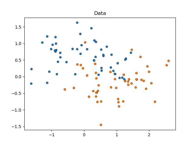
我们将首先模拟月牙形数据(其中类之间的理想分离是非线性的),并添加适度的噪声。数据点将属于两个可能的类别之一,由两个特征预测。我们将为每个类别模拟 50 个样本。
import matplotlib.pyplot as plt
import seaborn as sns

from sklearn.datasets import make_moons

X, y = make_moons(noise=0.352, random_state=1, n_samples=100)

sns.scatterplot(
    x=X[:, 0], y=X[:, 1], hue=y, marker="o", s=25, edgecolor="k", legend=False
).set_title("Data")
plt.show()
我们将比较 SVC 估计器在 kernel 参数上的性能,以决定哪种超参数选择能最好地预测我们模拟的数据。我们将使用 RepeatedStratifiedKFold 评估模型性能,重复 10 次 10 折分层交叉验证,每次重复使用不同的数据随机化。性能将使用 roc_auc_score 进行评估。
from sklearn.model_selection import GridSearchCV, RepeatedStratifiedKFold
from sklearn.svm import SVC

param_grid = [
    {"kernel": ["linear"]},
    {"kernel": ["poly"], "degree": [2, 3]},
    {"kernel": ["rbf"]},
]

svc = SVC(random_state=0)

cv = RepeatedStratifiedKFold(n_splits=10, n_repeats=10, random_state=0)

search = GridSearchCV(estimator=svc, param_grid=param_grid, scoring="roc_auc", cv=cv)
search.fit(X, y)
我们现在可以检查搜索结果,按 mean_test_score 排序
import pandas as pd

results_df = pd.DataFrame(search.cv_results_)
results_df = results_df.sort_values(by=["rank_test_score"])
results_df = results_df.set_index(
    results_df["params"].apply(lambda x: "_".join(str(val) for val in x.values()))
).rename_axis("kernel")
results_df[["params", "rank_test_score", "mean_test_score", "std_test_score"]]
我们可以看到使用 'rbf' 核的估计器表现最好,紧随其后的是 'linear'。两个使用 'poly' 核的估计器表现较差,其中使用二次多项式的模型性能远低于所有其他模型。
通常,分析到此为止,但故事才讲了一半。GridSearchCV 的输出没有提供模型之间差异的确定性信息。我们不知道这些差异是否具有**统计**显著性。为了评估这一点,我们需要进行统计检验。具体来说,为了对比两个模型的性能,我们应该统计比较它们的 AUC 分数。每个模型有 100 个样本(AUC 分数),因为我们重复了 10 次 10 折交叉验证。
然而,模型的得分并非独立:所有模型都在**相同**的 100 个分区上进行评估,这增加了模型性能之间的相关性。由于数据的某些分区可能使所有模型区分类别变得特别容易或困难,因此模型得分将共同变化。
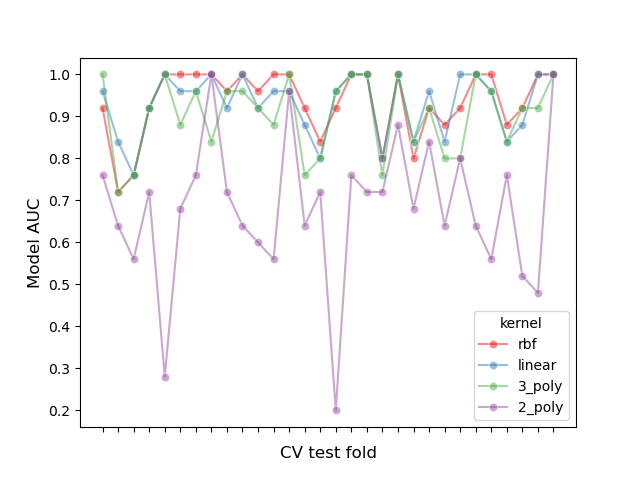
让我们通过绘制每个折叠中所有模型的性能,并计算折叠之间模型的相关性来检查这种分区效应
# create df of model scores ordered by performance
model_scores = results_df.filter(regex=r"split\d*_test_score")

# plot 30 examples of dependency between cv fold and AUC scores
fig, ax = plt.subplots()
sns.lineplot(
    data=model_scores.transpose().iloc[:30],
    dashes=False,
    palette="Set1",
    marker="o",
    alpha=0.5,
    ax=ax,
)
ax.set_xlabel("CV test fold", size=12, labelpad=10)
ax.set_ylabel("Model AUC", size=12)
ax.tick_params(bottom=True, labelbottom=False)
plt.show()

# print correlation of AUC scores across folds
print(f"Correlation of models:\n {model_scores.transpose().corr()}")
Correlation of models:
 kernel       rbf    linear    3_poly    2_poly
kernel
rbf     1.000000  0.882561  0.783392  0.351390
linear  0.882561  1.000000  0.746492  0.298688
3_poly  0.783392  0.746492  1.000000  0.355440
2_poly  0.351390  0.298688  0.355440  1.000000
我们可以观察到模型的性能高度依赖于折叠。
因此,如果我们假设样本之间相互独立,我们将低估统计检验中计算出的方差,从而增加假阳性错误的数量(即,当模型之间不存在显著差异时,却检测到显著差异) [1]。
针对这些情况,已经开发了几种方差校正的统计检验。在此示例中,我们将展示如何在两种不同的统计框架下实现其中一种(即 Nadeau 和 Bengio 校正的 t 检验):频率派和贝叶斯派。
比较两个模型:频率派方法#
我们可以首先问:“第一个模型是否比第二个模型(按 mean_test_score 排名时)显著更好?”
为了使用频率派方法回答这个问题,我们可以运行配对 t 检验并计算 p 值。这在预测文献中也称为 Diebold-Mariano 检验 [5]。已经开发了许多 t 检验变体来解决上一节中描述的“样本非独立性问题”。我们将使用一种经证明能获得最高可复现性分数(衡量模型在相同数据集的不同随机分区上评估时性能相似程度)同时保持低假阳性率和假阴性率的方法:即 Nadeau 和 Bengio 校正的 t 检验 [2],该检验使用 10 次重复的 10 折交叉验证 [3]。
这个校正后的配对 t 检验计算如下
其中 \(k\) 是折叠数,\(r\) 是交叉验证中的重复次数,\(x\) 是模型性能的差异,\(n_{test}\) 是用于测试的样本数量,\(n_{train}\) 是用于训练的样本数量,\(\hat{\sigma}^2\) 表示观察到的差异的方差。
让我们实现一个校正后的右尾配对 t 检验,以评估第一个模型的性能是否显著优于第二个模型。我们的零假设是第二个模型的性能至少与第一个模型一样好。
import numpy as np
from scipy.stats import t


def corrected_std(differences, n_train, n_test):
    """Corrects standard deviation using Nadeau and Bengio's approach.

    Parameters
    ----------
    differences : ndarray of shape (n_samples,)
        Vector containing the differences in the score metrics of two models.
    n_train : int
        Number of samples in the training set.
    n_test : int
        Number of samples in the testing set.

    Returns
    -------
    corrected_std : float
        Variance-corrected standard deviation of the set of differences.
    """
    # kr = k times r, r times repeated k-fold crossvalidation,
    # kr equals the number of times the model was evaluated
    kr = len(differences)
    corrected_var = np.var(differences, ddof=1) * (1 / kr + n_test / n_train)
    corrected_std = np.sqrt(corrected_var)
    return corrected_std


def compute_corrected_ttest(differences, df, n_train, n_test):
    """Computes right-tailed paired t-test with corrected variance.

    Parameters
    ----------
    differences : array-like of shape (n_samples,)
        Vector containing the differences in the score metrics of two models.
    df : int
        Degrees of freedom.
    n_train : int
        Number of samples in the training set.
    n_test : int
        Number of samples in the testing set.

    Returns
    -------
    t_stat : float
        Variance-corrected t-statistic.
    p_val : float
        Variance-corrected p-value.
    """
    mean = np.mean(differences)
    std = corrected_std(differences, n_train, n_test)
    t_stat = mean / std
    p_val = t.sf(np.abs(t_stat), df)  # right-tailed t-test
    return t_stat, p_val
model_1_scores = model_scores.iloc[0].values  # scores of the best model
model_2_scores = model_scores.iloc[1].values  # scores of the second-best model

differences = model_1_scores - model_2_scores

n = differences.shape[0]  # number of test sets
df = n - 1
n_train = len(next(iter(cv.split(X, y)))[0])
n_test = len(next(iter(cv.split(X, y)))[1])

t_stat, p_val = compute_corrected_ttest(differences, df, n_train, n_test)
print(f"Corrected t-value: {t_stat:.3f}\nCorrected p-value: {p_val:.3f}")
Corrected t-value: 0.750
Corrected p-value: 0.227
我们可以将校正后的 t 值和 p 值与未校正的值进行比较
Uncorrected t-value: 2.611
Uncorrected p-value: 0.005
使用传统的显著性 alpha 水平 p=0.05,我们观察到未校正的 t 检验得出结论:第一个模型显著优于第二个模型。
相比之下,使用校正方法,我们未能检测到这种差异。
然而,在后一种情况下,频率派方法不允许我们得出第一个模型和第二个模型具有等效性能的结论。如果我们要做出这种断言,我们需要使用贝叶斯方法。
比较两个模型:贝叶斯方法#
我们可以使用贝叶斯估计来计算第一个模型优于第二个模型的概率。贝叶斯估计将输出一个分布,其后是两个模型性能差异的均值 \(\mu\)。
为了获得后验分布,我们需要定义一个先验,该先验对在查看数据之前我们对均值分布的信念进行建模,并将其乘以一个似然函数,该函数计算给定均值差异可能取的值时,我们观察到的差异有多大可能性。
贝叶斯估计可以以多种形式进行以回答我们的问题,但在此示例中,我们将实现 Benavoli 及其同事提出的方法 [4]。
使用闭式表达式定义后验的一种方法是选择与似然函数共轭的先验。Benavoli 及其同事 [4] 表明,在比较两个分类器的性能时,我们可以将先验建模为与正态似然共轭的正态-伽马分布(均值和方差均未知),从而将后验表示为正态分布。从这个正态后验中边缘化掉方差,我们可以将均值参数的后验定义为学生 t 分布。具体来说
其中 \(n\) 是样本总数,\(\overline{x}\) 表示得分的平均差异,\(n_{test}\) 是用于测试的样本数量,\(n_{train}\) 是用于训练的样本数量,\(\hat{\sigma}^2\) 表示观察到的差异的方差。
请注意,我们在贝叶斯方法中也使用了 Nadeau 和 Bengio 的校正方差。
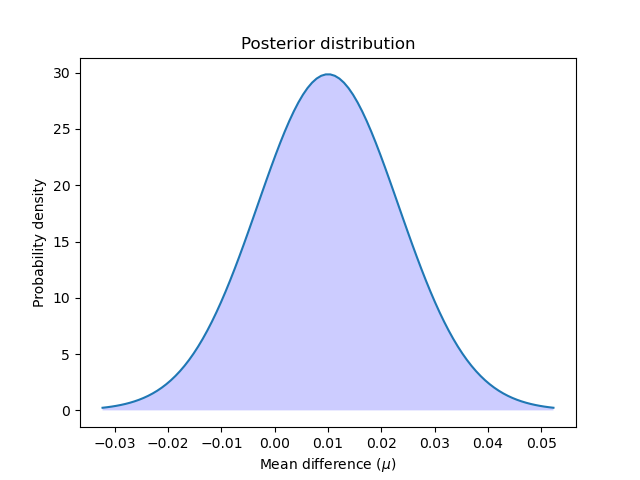
让我们计算并绘制后验
让我们绘制后验分布
x = np.linspace(t_post.ppf(0.001), t_post.ppf(0.999), 100)

plt.plot(x, t_post.pdf(x))
plt.xticks(np.arange(-0.04, 0.06, 0.01))
plt.fill_between(x, t_post.pdf(x), 0, facecolor="blue", alpha=0.2)
plt.ylabel("Probability density")
plt.xlabel(r"Mean difference ($\mu$)")
plt.title("Posterior distribution")
plt.show()
我们可以通过计算后验分布曲线从零到无穷大的面积来计算第一个模型优于第二个模型的概率。反之亦然:我们可以通过计算曲线从负无穷大到零的面积来计算第二个模型优于第一个模型的概率。
better_prob = 1 - t_post.cdf(0)

print(
    f"Probability of {model_scores.index[0]} being more accurate than "
    f"{model_scores.index[1]}: {better_prob:.3f}"
)
print(
    f"Probability of {model_scores.index[1]} being more accurate than "
    f"{model_scores.index[0]}: {1 - better_prob:.3f}"
)
Probability of rbf being more accurate than linear: 0.773
Probability of linear being more accurate than rbf: 0.227
与频率派方法相反,我们可以计算一个模型优于另一个模型的概率。
请注意,我们获得了与频率派方法相似的结果。考虑到我们对先验的选择,我们本质上执行的是相同的计算,但我们被允许做出不同的断言。
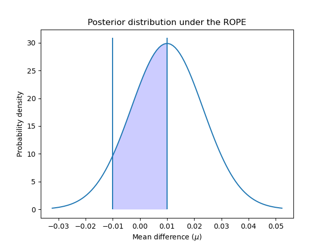
实际等效区域#
有时,我们对确定模型具有等效性能的概率感兴趣,其中“等效”以实际方式定义。一种朴素的方法 [4] 是将估计器定义为当其准确度差异小于 1% 时实际等效。但我们也可以根据我们试图解决的问题来定义这种实际等效。例如,准确度差异 5% 可能意味着销售额增加 1000 美元,我们认为任何高于此的量都与我们的业务相关。
在此示例中,我们将把实际等效区域 (ROPE) 定义为 \([-0.01, 0.01]\)。也就是说,如果两个模型的性能差异小于 1%,我们将认为它们实际等效。
为了计算分类器实际等效的概率,我们计算后验在 ROPE 区间下的曲线面积
rope_interval = [-0.01, 0.01]
rope_prob = t_post.cdf(rope_interval[1]) - t_post.cdf(rope_interval[0])

print(
    f"Probability of {model_scores.index[0]} and {model_scores.index[1]} "
    f"being practically equivalent: {rope_prob:.3f}"
)
Probability of rbf and linear being practically equivalent: 0.432
我们可以绘制后验在 ROPE 区间上的分布情况
x_rope = np.linspace(rope_interval[0], rope_interval[1], 100)

plt.plot(x, t_post.pdf(x))
plt.xticks(np.arange(-0.04, 0.06, 0.01))
plt.vlines([-0.01, 0.01], ymin=0, ymax=(np.max(t_post.pdf(x)) + 1))
plt.fill_between(x_rope, t_post.pdf(x_rope), 0, facecolor="blue", alpha=0.2)
plt.ylabel("Probability density")
plt.xlabel(r"Mean difference ($\mu$)")
plt.title("Posterior distribution under the ROPE")
plt.show()
如 [4] 中所建议,我们可以使用与频率派方法相同的标准进一步解释这些概率:落入 ROPE 内部的概率是否大于 95%(alpha 值为 5%)?在这种情况下,我们可以得出结论,两个模型实际等效。
贝叶斯估计方法还允许我们计算我们对差异估计的不确定性。这可以使用可信区间来计算。对于给定的概率,它们显示了估计量(在本例中为性能的平均差异)可以取的值的范围。例如,50% 的可信区间 [x, y] 告诉我们,模型之间真实(平均)性能差异在 x 和 y 之间的概率为 50%。
让我们使用 50%、75% 和 95% 确定数据的可信区间
cred_intervals = []
intervals = [0.5, 0.75, 0.95]

for interval in intervals:
    cred_interval = list(t_post.interval(interval))
    cred_intervals.append([interval, cred_interval[0], cred_interval[1]])

cred_int_df = pd.DataFrame(
    cred_intervals, columns=["interval", "lower value", "upper value"]
).set_index("interval")
cred_int_df
如表中所示,模型之间真实平均差异在 0.000977 和 0.019023 之间的概率为 50%,在 -0.005422 和 0.025422 之间的概率为 70%,在 -0.016445 和 0.036445 之间的概率为 95%。
所有模型的成对比较:频率派方法#
我们可能还对比较使用 GridSearchCV 评估的所有模型的性能感兴趣。在这种情况下,我们将多次运行我们的统计检验,这导致了多重比较问题。
解决这个问题有许多可能的方法,但一种标准方法是应用邦弗罗尼校正。邦弗罗尼校正可以通过将 p 值乘以我们正在检验的比较次数来计算。
让我们使用校正 t 检验比较模型的性能
from itertools import combinations
from math import factorial

n_comparisons = factorial(len(model_scores)) / (
    factorial(2) * factorial(len(model_scores) - 2)
)
pairwise_t_test = []

for model_i, model_k in combinations(range(len(model_scores)), 2):
    model_i_scores = model_scores.iloc[model_i].values
    model_k_scores = model_scores.iloc[model_k].values
    differences = model_i_scores - model_k_scores
    t_stat, p_val = compute_corrected_ttest(differences, df, n_train, n_test)
    p_val *= n_comparisons  # implement Bonferroni correction
    # Bonferroni can output p-values higher than 1
    p_val = 1 if p_val > 1 else p_val
    pairwise_t_test.append(
        [model_scores.index[model_i], model_scores.index[model_k], t_stat, p_val]
    )

pairwise_comp_df = pd.DataFrame(
    pairwise_t_test, columns=["model_1", "model_2", "t_stat", "p_val"]
).round(3)
pairwise_comp_df
我们观察到,在进行多重比较校正后,唯一与其他模型显著不同的模型是 '2_poly'。由 GridSearchCV 排名第一的模型 'rbf' 与 'linear' 或 '3_poly' 没有显著差异。
所有模型的成对比较:贝叶斯方法#
当使用贝叶斯估计比较多个模型时,我们不需要进行多重比较校正(原因请参见 [4])。
我们可以按照第一节中的相同方式进行成对比较
pairwise_bayesian = []

for model_i, model_k in combinations(range(len(model_scores)), 2):
    model_i_scores = model_scores.iloc[model_i].values
    model_k_scores = model_scores.iloc[model_k].values
    differences = model_i_scores - model_k_scores
    t_post = t(
        df, loc=np.mean(differences), scale=corrected_std(differences, n_train, n_test)
    )
    worse_prob = t_post.cdf(rope_interval[0])
    better_prob = 1 - t_post.cdf(rope_interval[1])
    rope_prob = t_post.cdf(rope_interval[1]) - t_post.cdf(rope_interval[0])

    pairwise_bayesian.append([worse_prob, better_prob, rope_prob])

pairwise_bayesian_df = pd.DataFrame(
    pairwise_bayesian, columns=["worse_prob", "better_prob", "rope_prob"]
).round(3)

pairwise_comp_df = pairwise_comp_df.join(pairwise_bayesian_df)
pairwise_comp_df
使用贝叶斯方法,我们可以计算一个模型性能优于、劣于或实际等效于另一个模型的概率。
结果显示,由 GridSearchCV 排名第一的模型 'rbf',其性能比 'linear' 差的概率约为 6.8%,比 '3_poly' 差的概率为 1.8%。'rbf' 和 'linear' 有 43% 的概率实际等效,而 'rbf' 和 '3_poly' 有 10% 的概率实际等效。
与使用频率派方法得出的结论类似,所有模型都有 100% 的概率优于 '2_poly',并且没有一个模型与后者具有实际等效的性能。
要点总结#
性能度量上的微小差异可能很容易仅仅是偶然的,而不是因为一个模型系统性地优于另一个。如本例所示,统计学可以告诉你这种情况发生的可能性有多大。
在 GridSearchCV 中统计比较两个模型的性能时,需要校正计算出的方差,因为模型的得分彼此不独立,这可能导致方差被低估。
使用(方差校正的)配对 t 检验的频率派方法可以告诉我们一个模型的性能是否以高于偶然的确定性优于另一个模型。
贝叶斯方法可以提供一个模型优于、劣于或实际等效于另一个模型的概率。它还可以告诉我们,我们有多大信心知道模型的真实差异落在某个值范围内。
如果对多个模型进行统计比较,使用频率派方法时需要进行多重比较校正。
参考文献
脚本总运行时间: (0 分 1.514 秒)
相关示例