文本文档的核外分类#

此示例展示了 scikit-learn 如何使用核外方法进行分类：从不适合主内存的数据中学习。我们使用了一个在线分类器，即支持 partial_fit 方法的分类器，它将分批接收示例。为了保证特征空间随时间保持不变，我们利用 HashingVectorizer 将每个示例投影到相同的特征空间中。这在文本分类中特别有用，因为每个批次中都可能出现新特征（词）。

# Authors: The scikit-learn developers
# SPDX-License-Identifier: BSD-3-Clause

import itertools
import re
import sys
import tarfile
import time
from hashlib import sha256
from html.parser import HTMLParser
from pathlib import Path
from urllib.request import urlretrieve

import matplotlib.pyplot as plt
import numpy as np
from matplotlib import rcParams

from sklearn.datasets import get_data_home
from sklearn.feature_extraction.text import HashingVectorizer
from sklearn.linear_model import PassiveAggressiveClassifier, Perceptron, SGDClassifier
from sklearn.naive_bayes import MultinomialNB


def _not_in_sphinx():
    # Hack to detect whether we are running by the sphinx builder
    return "__file__" in globals()

Reuters 数据集相关例程#

此示例中使用的数据集是 UCI ML 仓库提供的 Reuters-21578。首次运行时将自动下载并解压缩。

class ReutersParser(HTMLParser):
    """Utility class to parse a SGML file and yield documents one at a time."""

    def __init__(self, encoding="latin-1"):
        HTMLParser.__init__(self)
        self._reset()
        self.encoding = encoding

    def handle_starttag(self, tag, attrs):
        method = "start_" + tag
        getattr(self, method, lambda x: None)(attrs)

    def handle_endtag(self, tag):
        method = "end_" + tag
        getattr(self, method, lambda: None)()

    def _reset(self):
        self.in_title = 0
        self.in_body = 0
        self.in_topics = 0
        self.in_topic_d = 0
        self.title = ""
        self.body = ""
        self.topics = []
        self.topic_d = ""

    def parse(self, fd):
        self.docs = []
        for chunk in fd:
            self.feed(chunk.decode(self.encoding))
            for doc in self.docs:
                yield doc
            self.docs = []
        self.close()

    def handle_data(self, data):
        if self.in_body:
            self.body += data
        elif self.in_title:
            self.title += data
        elif self.in_topic_d:
            self.topic_d += data

    def start_reuters(self, attributes):
        pass

    def end_reuters(self):
        self.body = re.sub(r"\s+", r" ", self.body)
        self.docs.append(
            {"title": self.title, "body": self.body, "topics": self.topics}
        )
        self._reset()

    def start_title(self, attributes):
        self.in_title = 1

    def end_title(self):
        self.in_title = 0

    def start_body(self, attributes):
        self.in_body = 1

    def end_body(self):
        self.in_body = 0

    def start_topics(self, attributes):
        self.in_topics = 1

    def end_topics(self):
        self.in_topics = 0

    def start_d(self, attributes):
        self.in_topic_d = 1

    def end_d(self):
        self.in_topic_d = 0
        self.topics.append(self.topic_d)
        self.topic_d = ""


def stream_reuters_documents(data_path=None):
    """Iterate over documents of the Reuters dataset.

    The Reuters archive will automatically be downloaded and uncompressed if
    the `data_path` directory does not exist.

    Documents are represented as dictionaries with 'body' (str),
    'title' (str), 'topics' (list(str)) keys.

    """

    DOWNLOAD_URL = "https://kdd.ics.uci.edu/databases/reuters21578/reuters21578.tar.gz"
    ARCHIVE_SHA256 = "3bae43c9b14e387f76a61b6d82bf98a4fb5d3ef99ef7e7075ff2ccbcf59f9d30"
    ARCHIVE_FILENAME = "reuters21578.tar.gz"

    if data_path is None:
        data_path = Path(get_data_home()) / "reuters"
    else:
        data_path = Path(data_path)
    if not data_path.exists():
        """Download the dataset."""
        print("downloading dataset (once and for all) into %s" % data_path)
        data_path.mkdir(parents=True, exist_ok=True)

        def progress(blocknum, bs, size):
            total_sz_mb = "%.2f MB" % (size / 1e6)
            current_sz_mb = "%.2f MB" % ((blocknum * bs) / 1e6)
            if _not_in_sphinx():
                sys.stdout.write("\rdownloaded %s / %s" % (current_sz_mb, total_sz_mb))

        archive_path = data_path / ARCHIVE_FILENAME

        urlretrieve(DOWNLOAD_URL, filename=archive_path, reporthook=progress)
        if _not_in_sphinx():
            sys.stdout.write("\r")

        # Check that the archive was not tampered:
        assert sha256(archive_path.read_bytes()).hexdigest() == ARCHIVE_SHA256

        print("untarring Reuters dataset...")
        with tarfile.open(archive_path, "r:gz") as fp:
            fp.extractall(data_path, filter="data")
        print("done.")

    parser = ReutersParser()
    for filename in data_path.glob("*.sgm"):
        for doc in parser.parse(open(filename, "rb")):
            yield doc

主程序#

创建向量化器并限制特征数量到一个合理的上限

vectorizer = HashingVectorizer(
    decode_error="ignore", n_features=2**18, alternate_sign=False
)


# Iterator over parsed Reuters SGML files.
data_stream = stream_reuters_documents()

# We learn a binary classification between the "acq" class and all the others.
# "acq" was chosen as it is more or less evenly distributed in the Reuters
# files. For other datasets, one should take care of creating a test set with
# a realistic portion of positive instances.
all_classes = np.array([0, 1])
positive_class = "acq"

# Here are some classifiers that support the `partial_fit` method
partial_fit_classifiers = {
    "SGD": SGDClassifier(max_iter=5),
    "Perceptron": Perceptron(),
    "NB Multinomial": MultinomialNB(alpha=0.01),
    "Passive-Aggressive": PassiveAggressiveClassifier(),
}


def get_minibatch(doc_iter, size, pos_class=positive_class):
    """Extract a minibatch of examples, return a tuple X_text, y.

    Note: size is before excluding invalid docs with no topics assigned.

    """
    data = [
        ("{title}\n\n{body}".format(**doc), pos_class in doc["topics"])
        for doc in itertools.islice(doc_iter, size)
        if doc["topics"]
    ]
    if not len(data):
        return np.asarray([], dtype=int), np.asarray([], dtype=int)
    X_text, y = zip(*data)
    return X_text, np.asarray(y, dtype=int)


def iter_minibatches(doc_iter, minibatch_size):
    """Generator of minibatches."""
    X_text, y = get_minibatch(doc_iter, minibatch_size)
    while len(X_text):
        yield X_text, y
        X_text, y = get_minibatch(doc_iter, minibatch_size)


# test data statistics
test_stats = {"n_test": 0, "n_test_pos": 0}

# First we hold out a number of examples to estimate accuracy
n_test_documents = 1000
tick = time.time()
X_test_text, y_test = get_minibatch(data_stream, 1000)
parsing_time = time.time() - tick
tick = time.time()
X_test = vectorizer.transform(X_test_text)
vectorizing_time = time.time() - tick
test_stats["n_test"] += len(y_test)
test_stats["n_test_pos"] += sum(y_test)
print("Test set is %d documents (%d positive)" % (len(y_test), sum(y_test)))


def progress(cls_name, stats):
    """Report progress information, return a string."""
    duration = time.time() - stats["t0"]
    s = "%20s classifier : \t" % cls_name
    s += "%(n_train)6d train docs (%(n_train_pos)6d positive) " % stats
    s += "%(n_test)6d test docs (%(n_test_pos)6d positive) " % test_stats
    s += "accuracy: %(accuracy).3f " % stats
    s += "in %.2fs (%5d docs/s)" % (duration, stats["n_train"] / duration)
    return s


cls_stats = {}

for cls_name in partial_fit_classifiers:
    stats = {
        "n_train": 0,
        "n_train_pos": 0,
        "accuracy": 0.0,
        "accuracy_history": [(0, 0)],
        "t0": time.time(),
        "runtime_history": [(0, 0)],
        "total_fit_time": 0.0,
    }
    cls_stats[cls_name] = stats

get_minibatch(data_stream, n_test_documents)
# Discard test set

# We will feed the classifier with mini-batches of 1000 documents; this means
# we have at most 1000 docs in memory at any time.  The smaller the document
# batch, the bigger the relative overhead of the partial fit methods.
minibatch_size = 1000

# Create the data_stream that parses Reuters SGML files and iterates on
# documents as a stream.
minibatch_iterators = iter_minibatches(data_stream, minibatch_size)
total_vect_time = 0.0

# Main loop : iterate on mini-batches of examples
for i, (X_train_text, y_train) in enumerate(minibatch_iterators):
    tick = time.time()
    X_train = vectorizer.transform(X_train_text)
    total_vect_time += time.time() - tick

    for cls_name, cls in partial_fit_classifiers.items():
        tick = time.time()
        # update estimator with examples in the current mini-batch
        cls.partial_fit(X_train, y_train, classes=all_classes)

        # accumulate test accuracy stats
        cls_stats[cls_name]["total_fit_time"] += time.time() - tick
        cls_stats[cls_name]["n_train"] += X_train.shape[0]
        cls_stats[cls_name]["n_train_pos"] += sum(y_train)
        tick = time.time()
        cls_stats[cls_name]["accuracy"] = cls.score(X_test, y_test)
        cls_stats[cls_name]["prediction_time"] = time.time() - tick
        acc_history = (cls_stats[cls_name]["accuracy"], cls_stats[cls_name]["n_train"])
        cls_stats[cls_name]["accuracy_history"].append(acc_history)
        run_history = (
            cls_stats[cls_name]["accuracy"],
            total_vect_time + cls_stats[cls_name]["total_fit_time"],
        )
        cls_stats[cls_name]["runtime_history"].append(run_history)

        if i % 3 == 0:
            print(progress(cls_name, cls_stats[cls_name]))
    if i % 3 == 0:
        print("\n")

Test set is 878 documents (108 positive)
                 SGD classifier :          962 train docs (   132 positive)    878 test docs (   108 positive) accuracy: 0.915 in 0.65s ( 1470 docs/s)
          Perceptron classifier :          962 train docs (   132 positive)    878 test docs (   108 positive) accuracy: 0.855 in 0.66s ( 1462 docs/s)
      NB Multinomial classifier :          962 train docs (   132 positive)    878 test docs (   108 positive) accuracy: 0.877 in 0.67s ( 1442 docs/s)
  Passive-Aggressive classifier :          962 train docs (   132 positive)    878 test docs (   108 positive) accuracy: 0.933 in 0.67s ( 1435 docs/s)


                 SGD classifier :         3911 train docs (   517 positive)    878 test docs (   108 positive) accuracy: 0.938 in 1.82s ( 2148 docs/s)
          Perceptron classifier :         3911 train docs (   517 positive)    878 test docs (   108 positive) accuracy: 0.936 in 1.82s ( 2145 docs/s)
      NB Multinomial classifier :         3911 train docs (   517 positive)    878 test docs (   108 positive) accuracy: 0.885 in 1.83s ( 2135 docs/s)
  Passive-Aggressive classifier :         3911 train docs (   517 positive)    878 test docs (   108 positive) accuracy: 0.941 in 1.83s ( 2131 docs/s)


                 SGD classifier :         6821 train docs (   891 positive)    878 test docs (   108 positive) accuracy: 0.952 in 2.97s ( 2298 docs/s)
          Perceptron classifier :         6821 train docs (   891 positive)    878 test docs (   108 positive) accuracy: 0.952 in 2.97s ( 2296 docs/s)
      NB Multinomial classifier :         6821 train docs (   891 positive)    878 test docs (   108 positive) accuracy: 0.900 in 2.98s ( 2290 docs/s)
  Passive-Aggressive classifier :         6821 train docs (   891 positive)    878 test docs (   108 positive) accuracy: 0.953 in 2.98s ( 2288 docs/s)


                 SGD classifier :         9759 train docs (  1276 positive)    878 test docs (   108 positive) accuracy: 0.949 in 4.12s ( 2366 docs/s)
          Perceptron classifier :         9759 train docs (  1276 positive)    878 test docs (   108 positive) accuracy: 0.953 in 4.13s ( 2364 docs/s)
      NB Multinomial classifier :         9759 train docs (  1276 positive)    878 test docs (   108 positive) accuracy: 0.909 in 4.14s ( 2359 docs/s)
  Passive-Aggressive classifier :         9759 train docs (  1276 positive)    878 test docs (   108 positive) accuracy: 0.958 in 4.14s ( 2357 docs/s)


                 SGD classifier :        11680 train docs (  1499 positive)    878 test docs (   108 positive) accuracy: 0.944 in 5.11s ( 2284 docs/s)
          Perceptron classifier :        11680 train docs (  1499 positive)    878 test docs (   108 positive) accuracy: 0.956 in 5.12s ( 2282 docs/s)
      NB Multinomial classifier :        11680 train docs (  1499 positive)    878 test docs (   108 positive) accuracy: 0.915 in 5.12s ( 2279 docs/s)
  Passive-Aggressive classifier :        11680 train docs (  1499 positive)    878 test docs (   108 positive) accuracy: 0.950 in 5.13s ( 2278 docs/s)


                 SGD classifier :        14625 train docs (  1865 positive)    878 test docs (   108 positive) accuracy: 0.965 in 6.38s ( 2292 docs/s)
          Perceptron classifier :        14625 train docs (  1865 positive)    878 test docs (   108 positive) accuracy: 0.903 in 6.38s ( 2291 docs/s)
      NB Multinomial classifier :        14625 train docs (  1865 positive)    878 test docs (   108 positive) accuracy: 0.924 in 6.39s ( 2288 docs/s)
  Passive-Aggressive classifier :        14625 train docs (  1865 positive)    878 test docs (   108 positive) accuracy: 0.957 in 6.39s ( 2287 docs/s)


                 SGD classifier :        17360 train docs (  2179 positive)    878 test docs (   108 positive) accuracy: 0.957 in 7.44s ( 2334 docs/s)
          Perceptron classifier :        17360 train docs (  2179 positive)    878 test docs (   108 positive) accuracy: 0.933 in 7.44s ( 2333 docs/s)
      NB Multinomial classifier :        17360 train docs (  2179 positive)    878 test docs (   108 positive) accuracy: 0.932 in 7.45s ( 2330 docs/s)
  Passive-Aggressive classifier :        17360 train docs (  2179 positive)    878 test docs (   108 positive) accuracy: 0.952 in 7.45s ( 2329 docs/s)

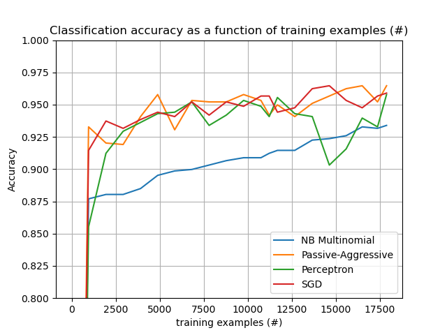
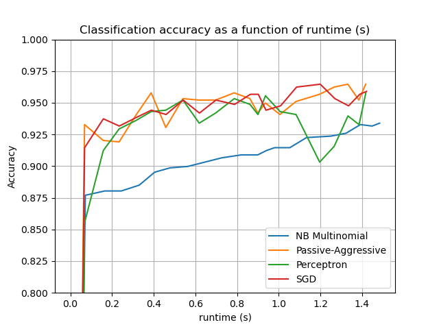
绘制结果#

该图表示分类器的学习曲线：分类精度在小批次过程中的演变。精度是在前 1000 个样本（作为验证集保留）上测量的。

为了限制内存消耗，我们在将示例送入学习器之前，将它们排队到固定数量。

def plot_accuracy(x, y, x_legend):
    """Plot accuracy as a function of x."""
    x = np.array(x)
    y = np.array(y)
    plt.title("Classification accuracy as a function of %s" % x_legend)
    plt.xlabel("%s" % x_legend)
    plt.ylabel("Accuracy")
    plt.grid(True)
    plt.plot(x, y)


rcParams["legend.fontsize"] = 10
cls_names = list(sorted(cls_stats.keys()))

# Plot accuracy evolution
plt.figure()
for _, stats in sorted(cls_stats.items()):
    # Plot accuracy evolution with #examples
    accuracy, n_examples = zip(*stats["accuracy_history"])
    plot_accuracy(n_examples, accuracy, "training examples (#)")
    ax = plt.gca()
    ax.set_ylim((0.8, 1))
plt.legend(cls_names, loc="best")

plt.figure()
for _, stats in sorted(cls_stats.items()):
    # Plot accuracy evolution with runtime
    accuracy, runtime = zip(*stats["runtime_history"])
    plot_accuracy(runtime, accuracy, "runtime (s)")
    ax = plt.gca()
    ax.set_ylim((0.8, 1))
plt.legend(cls_names, loc="best")

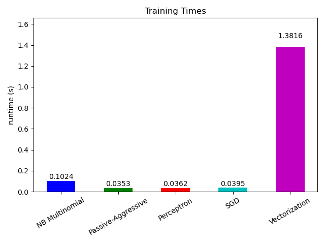
# Plot fitting times
plt.figure()
fig = plt.gcf()
cls_runtime = [stats["total_fit_time"] for cls_name, stats in sorted(cls_stats.items())]

cls_runtime.append(total_vect_time)
cls_names.append("Vectorization")
bar_colors = ["b", "g", "r", "c", "m", "y"]

ax = plt.subplot(111)
rectangles = plt.bar(range(len(cls_names)), cls_runtime, width=0.5, color=bar_colors)

ax.set_xticks(np.linspace(0, len(cls_names) - 1, len(cls_names)))
ax.set_xticklabels(cls_names, fontsize=10)
ymax = max(cls_runtime) * 1.2
ax.set_ylim((0, ymax))
ax.set_ylabel("runtime (s)")
ax.set_title("Training Times")


def autolabel(rectangles):
    """attach some text vi autolabel on rectangles."""
    for rect in rectangles:
        height = rect.get_height()
        ax.text(
            rect.get_x() + rect.get_width() / 2.0,
            1.05 * height,
            "%.4f" % height,
            ha="center",
            va="bottom",
        )
        plt.setp(plt.xticks()[1], rotation=30)


autolabel(rectangles)
plt.tight_layout()
plt.show()

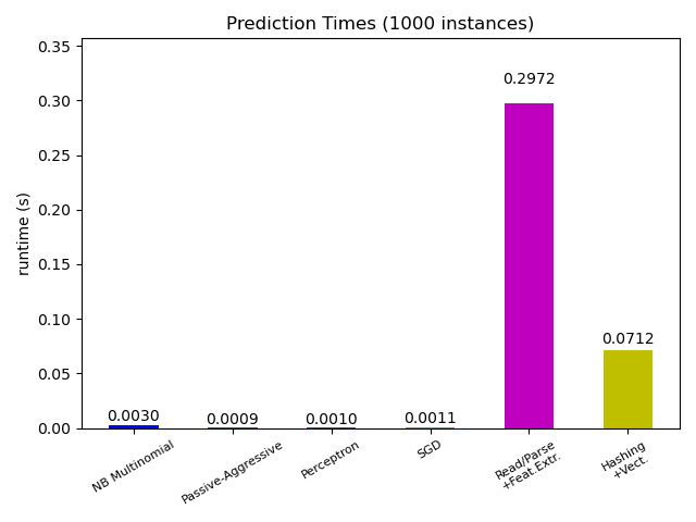
# Plot prediction times
plt.figure()
cls_runtime = []
cls_names = list(sorted(cls_stats.keys()))
for cls_name, stats in sorted(cls_stats.items()):
    cls_runtime.append(stats["prediction_time"])
cls_runtime.append(parsing_time)
cls_names.append("Read/Parse\n+Feat.Extr.")
cls_runtime.append(vectorizing_time)
cls_names.append("Hashing\n+Vect.")

ax = plt.subplot(111)
rectangles = plt.bar(range(len(cls_names)), cls_runtime, width=0.5, color=bar_colors)

ax.set_xticks(np.linspace(0, len(cls_names) - 1, len(cls_names)))
ax.set_xticklabels(cls_names, fontsize=8)
plt.setp(plt.xticks()[1], rotation=30)
ymax = max(cls_runtime) * 1.2
ax.set_ylim((0, ymax))
ax.set_ylabel("runtime (s)")
ax.set_title("Prediction Times (%d instances)" % n_test_documents)
autolabel(rectangles)
plt.tight_layout()
plt.show()