比较线性贝叶斯回归器#

此示例比较了两种不同的贝叶斯回归器

一个自动相关性确定 - ARD
一个贝叶斯岭回归

在第一部分中，我们使用一个普通最小二乘 (OLS) 模型作为基线，用于比较模型系数与真实系数的关系。此后，我们展示了这些模型的估计是通过迭代最大化观测值的边际对数似然来完成的。

在最后一部分中，我们使用多项式特征扩展来绘制 ARD 和贝叶斯岭回归的预测和不确定性，以拟合 X 和 y 之间的非线性关系。

# Authors: The scikit-learn developers
# SPDX-License-Identifier: BSD-3-Clause

模型恢复真实权重的鲁棒性#

生成合成数据集#

我们生成一个数据集，其中 X 和 y 线性关联：X 的 10 个特征将用于生成 y。其他特征对预测 y 没有用。此外，我们生成一个数据集，其中 n_samples == n_features。这种设置对 OLS 模型来说具有挑战性，并可能导致任意大的权重。对权重施加先验和惩罚可以缓解这个问题。最后，添加了高斯噪声。

from sklearn.datasets import make_regression

X, y, true_weights = make_regression(
    n_samples=100,
    n_features=100,
    n_informative=10,
    noise=8,
    coef=True,
    random_state=42,
)

拟合回归器#

我们现在拟合贝叶斯模型和 OLS，以便稍后比较模型的系数。

import pandas as pd

from sklearn.linear_model import ARDRegression, BayesianRidge, LinearRegression

olr = LinearRegression().fit(X, y)
brr = BayesianRidge(compute_score=True, max_iter=30).fit(X, y)
ard = ARDRegression(compute_score=True, max_iter=30).fit(X, y)
df = pd.DataFrame(
    {
        "Weights of true generative process": true_weights,
        "ARDRegression": ard.coef_,
        "BayesianRidge": brr.coef_,
        "LinearRegression": olr.coef_,
    }
)

绘制真实和估计的系数#

现在我们比较每个模型的系数与真实生成模型的权重。

import matplotlib.pyplot as plt
import seaborn as sns
from matplotlib.colors import SymLogNorm

plt.figure(figsize=(10, 6))
ax = sns.heatmap(
    df.T,
    norm=SymLogNorm(linthresh=10e-4, vmin=-80, vmax=80),
    cbar_kws={"label": "coefficients' values"},
    cmap="seismic_r",
)
plt.ylabel("linear model")
plt.xlabel("coefficients")
plt.tight_layout(rect=(0, 0, 1, 0.95))
_ = plt.title("Models' coefficients")

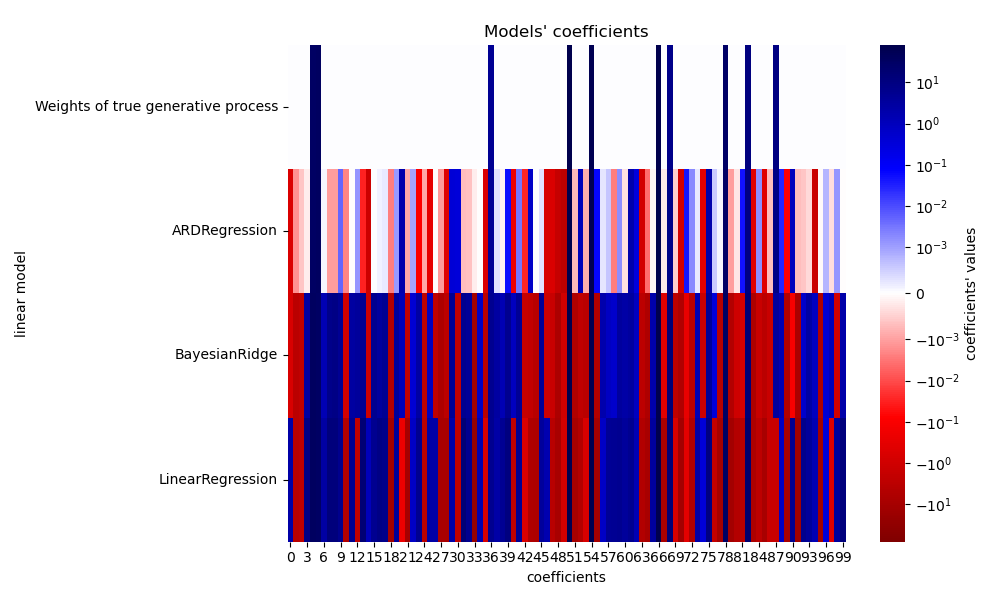
由于添加了噪声，没有一个模型能完全恢复真实权重。事实上，所有模型总是拥有超过 10 个非零系数。与 OLS 估计器相比，使用贝叶斯岭回归的系数略微向零移动，从而使其稳定。ARD 回归提供了一个更稀疏的解：一些非信息性系数被精确地设置为零，而其他系数则更接近于零。一些非信息性系数仍然存在并保留较大的值。

绘制边际对数似然#

import numpy as np

ard_scores = -np.array(ard.scores_)
brr_scores = -np.array(brr.scores_)
plt.plot(ard_scores, color="navy", label="ARD")
plt.plot(brr_scores, color="red", label="BayesianRidge")
plt.ylabel("Log-likelihood")
plt.xlabel("Iterations")
plt.xlim(1, 30)
plt.legend()
_ = plt.title("Models log-likelihood")

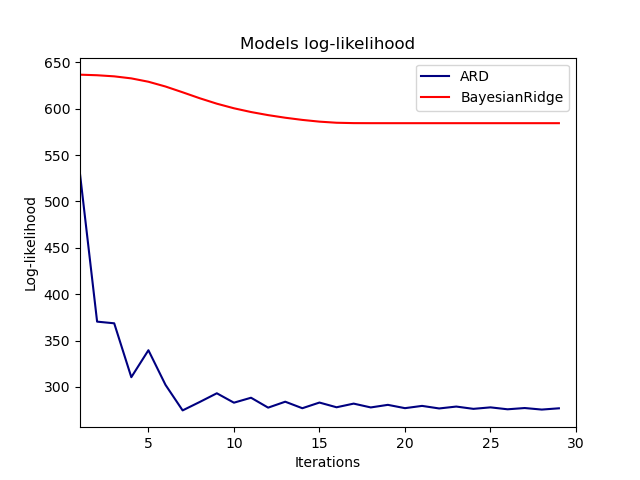
事实上，这两个模型都将对数似然最小化，直到达到由 max_iter 参数定义的任意截止值。

带多项式特征扩展的贝叶斯回归#

生成合成数据集#

我们创建一个目标，它是输入特征的非线性函数。添加了遵循标准均匀分布的噪声。

from sklearn.pipeline import make_pipeline
from sklearn.preprocessing import PolynomialFeatures, StandardScaler

rng = np.random.RandomState(0)
n_samples = 110

# sort the data to make plotting easier later
X = np.sort(-10 * rng.rand(n_samples) + 10)
noise = rng.normal(0, 1, n_samples) * 1.35
y = np.sqrt(X) * np.sin(X) + noise
full_data = pd.DataFrame({"input_feature": X, "target": y})
X = X.reshape((-1, 1))

# extrapolation
X_plot = np.linspace(10, 10.4, 10)
y_plot = np.sqrt(X_plot) * np.sin(X_plot)
X_plot = np.concatenate((X, X_plot.reshape((-1, 1))))
y_plot = np.concatenate((y - noise, y_plot))

拟合回归器#

在这里，我们尝试一个 10 次多项式，可能会导致过拟合，尽管贝叶斯线性模型会对多项式系数的大小进行正则化。由于 ARDRegression 和 BayesianRidge 默认 fit_intercept=True，因此 PolynomialFeatures 不应引入额外的偏差特征。通过设置 return_std=True，贝叶斯回归器会返回模型参数后验分布的标准差。

ard_poly = make_pipeline(
    PolynomialFeatures(degree=10, include_bias=False),
    StandardScaler(),
    ARDRegression(),
).fit(X, y)
brr_poly = make_pipeline(
    PolynomialFeatures(degree=10, include_bias=False),
    StandardScaler(),
    BayesianRidge(),
).fit(X, y)

y_ard, y_ard_std = ard_poly.predict(X_plot, return_std=True)
y_brr, y_brr_std = brr_poly.predict(X_plot, return_std=True)

绘制带分数标准误差的多项式回归#

ax = sns.scatterplot(
    data=full_data, x="input_feature", y="target", color="black", alpha=0.75
)
ax.plot(X_plot, y_plot, color="black", label="Ground Truth")
ax.plot(X_plot, y_brr, color="red", label="BayesianRidge with polynomial features")
ax.plot(X_plot, y_ard, color="navy", label="ARD with polynomial features")
ax.fill_between(
    X_plot.ravel(),
    y_ard - y_ard_std,
    y_ard + y_ard_std,
    color="navy",
    alpha=0.3,
)
ax.fill_between(
    X_plot.ravel(),
    y_brr - y_brr_std,
    y_brr + y_brr_std,
    color="red",
    alpha=0.3,
)
ax.legend()
_ = ax.set_title("Polynomial fit of a non-linear feature")

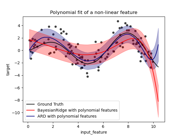
误差条表示查询点预测高斯分布的一个标准差。请注意，当在两个模型中使用默认参数时，ARD 回归能够最好地捕获真实值，但进一步降低贝叶斯岭的 lambda_init 超参数可以减少其偏差（参见示例使用贝叶斯岭回归进行曲线拟合）。最后，由于多项式回归的内在局限性，两个模型在进行外推时都会失败。

脚本总运行时间： (0 分 0.640 秒)

比较线性贝叶斯回归器#

模型恢复真实权重的鲁棒性#

生成合成数据集#

拟合回归器#

绘制真实和估计的系数#

绘制边际对数似然#

带多项式特征扩展的贝叶斯回归#

生成合成数据集#

拟合回归器#

绘制带分数标准误差的多项式回归#

本页