截断球体上的流形学习方法#

不同的流形学习技术在球形数据集上的应用。在这里，我们可以看到降维的使用是为了对流形学习方法获得一些直观理解。关于数据集，球体的两极以及侧面的一薄片被切除。这使得流形学习技术能够在投影到二维空间时“将其展开”。

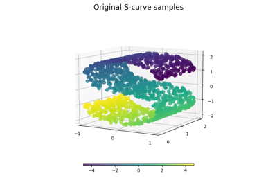
对于类似示例，其中方法应用于 S 曲线数据集，请参阅流形学习方法比较

请注意，MDS 的目的是找到数据的低维表示（此处为二维），其中距离能很好地尊重原始高维空间中的距离，与其他流形学习算法不同，它不寻求数据在低维空间中的各向同性表示。这里的流形问题与表示地球平面地图的问题相当匹配，例如地图投影

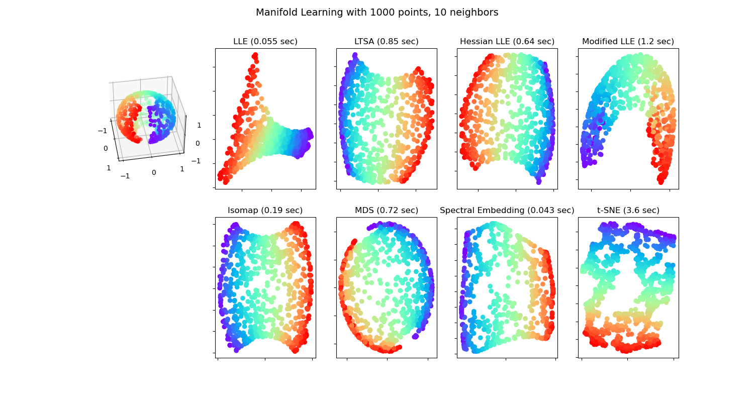
Manifold Learning with 1000 points, 10 neighbors, LLE (0.055 sec), LTSA (0.85 sec), Hessian LLE (0.64 sec), Modified LLE (1.2 sec), Isomap (0.19 sec), MDS (0.72 sec), Spectral Embedding (0.043 sec), t-SNE (3.6 sec)

standard: 0.055 sec
ltsa: 0.85 sec
hessian: 0.64 sec
modified: 1.2 sec
ISO: 0.19 sec
MDS: 0.72 sec
Spectral Embedding: 0.043 sec
t-SNE: 3.6 sec

# Authors: The scikit-learn developers
# SPDX-License-Identifier: BSD-3-Clause

from time import time

import matplotlib.pyplot as plt

# Unused but required import for doing 3d projections with matplotlib < 3.2
import mpl_toolkits.mplot3d  # noqa: F401
import numpy as np
from matplotlib.ticker import NullFormatter

from sklearn import manifold
from sklearn.utils import check_random_state

# Variables for manifold learning.
n_neighbors = 10
n_samples = 1000

# Create our sphere.
random_state = check_random_state(0)
p = random_state.rand(n_samples) * (2 * np.pi - 0.55)
t = random_state.rand(n_samples) * np.pi

# Sever the poles from the sphere.
indices = (t < (np.pi - (np.pi / 8))) & (t > (np.pi / 8))
colors = p[indices]
x, y, z = (
    np.sin(t[indices]) * np.cos(p[indices]),
    np.sin(t[indices]) * np.sin(p[indices]),
    np.cos(t[indices]),
)

# Plot our dataset.
fig = plt.figure(figsize=(15, 8))
plt.suptitle(
    "Manifold Learning with %i points, %i neighbors" % (1000, n_neighbors), fontsize=14
)

ax = fig.add_subplot(251, projection="3d")
ax.scatter(x, y, z, c=p[indices], cmap=plt.cm.rainbow)
ax.view_init(40, -10)

sphere_data = np.array([x, y, z]).T

# Perform Locally Linear Embedding Manifold learning
methods = ["standard", "ltsa", "hessian", "modified"]
labels = ["LLE", "LTSA", "Hessian LLE", "Modified LLE"]

for i, method in enumerate(methods):
    t0 = time()
    trans_data = (
        manifold.LocallyLinearEmbedding(
            n_neighbors=n_neighbors, n_components=2, method=method, random_state=42
        )
        .fit_transform(sphere_data)
        .T
    )
    t1 = time()
    print("%s: %.2g sec" % (methods[i], t1 - t0))

    ax = fig.add_subplot(252 + i)
    plt.scatter(trans_data[0], trans_data[1], c=colors, cmap=plt.cm.rainbow)
    plt.title("%s (%.2g sec)" % (labels[i], t1 - t0))
    ax.xaxis.set_major_formatter(NullFormatter())
    ax.yaxis.set_major_formatter(NullFormatter())
    plt.axis("tight")

# Perform Isomap Manifold learning.
t0 = time()
trans_data = (
    manifold.Isomap(n_neighbors=n_neighbors, n_components=2)
    .fit_transform(sphere_data)
    .T
)
t1 = time()
print("%s: %.2g sec" % ("ISO", t1 - t0))

ax = fig.add_subplot(257)
plt.scatter(trans_data[0], trans_data[1], c=colors, cmap=plt.cm.rainbow)
plt.title("%s (%.2g sec)" % ("Isomap", t1 - t0))
ax.xaxis.set_major_formatter(NullFormatter())
ax.yaxis.set_major_formatter(NullFormatter())
plt.axis("tight")

# Perform Multi-dimensional scaling.
t0 = time()
mds = manifold.MDS(2, max_iter=100, n_init=1, random_state=42)
trans_data = mds.fit_transform(sphere_data).T
t1 = time()
print("MDS: %.2g sec" % (t1 - t0))

ax = fig.add_subplot(258)
plt.scatter(trans_data[0], trans_data[1], c=colors, cmap=plt.cm.rainbow)
plt.title("MDS (%.2g sec)" % (t1 - t0))
ax.xaxis.set_major_formatter(NullFormatter())
ax.yaxis.set_major_formatter(NullFormatter())
plt.axis("tight")

# Perform Spectral Embedding.
t0 = time()
se = manifold.SpectralEmbedding(
    n_components=2, n_neighbors=n_neighbors, random_state=42
)
trans_data = se.fit_transform(sphere_data).T
t1 = time()
print("Spectral Embedding: %.2g sec" % (t1 - t0))

ax = fig.add_subplot(259)
plt.scatter(trans_data[0], trans_data[1], c=colors, cmap=plt.cm.rainbow)
plt.title("Spectral Embedding (%.2g sec)" % (t1 - t0))
ax.xaxis.set_major_formatter(NullFormatter())
ax.yaxis.set_major_formatter(NullFormatter())
plt.axis("tight")

# Perform t-distributed stochastic neighbor embedding.
t0 = time()
tsne = manifold.TSNE(n_components=2, random_state=0)
trans_data = tsne.fit_transform(sphere_data).T
t1 = time()
print("t-SNE: %.2g sec" % (t1 - t0))

ax = fig.add_subplot(2, 5, 10)
plt.scatter(trans_data[0], trans_data[1], c=colors, cmap=plt.cm.rainbow)
plt.title("t-SNE (%.2g sec)" % (t1 - t0))
ax.xaxis.set_major_formatter(NullFormatter())
ax.yaxis.set_major_formatter(NullFormatter())
plt.axis("tight")

plt.show()

脚本总运行时间： (0 分 7.901 秒)

截断球体上的流形学习方法#

本页