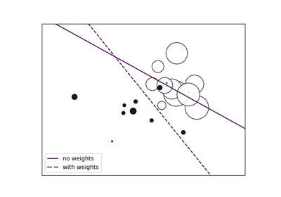
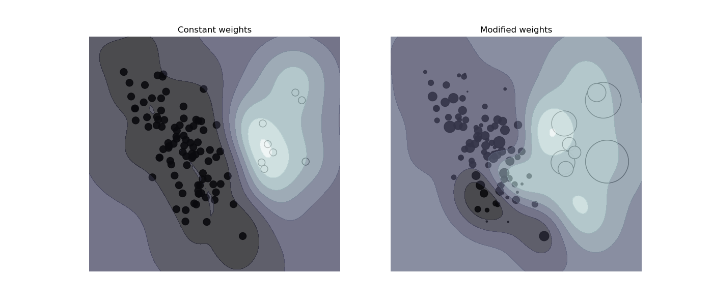
SVM：加权样本#

绘制加权数据集的决策函数，其中点的大小与其权重成比例。

样本加权重新缩放了C参数，这意味着分类器更强调正确处理这些点。效果可能通常很微妙。为了在此处强调这种效果，我们特别增加了正类的权重，使得决策边界的变形更加明显。

# Authors: The scikit-learn developers
# SPDX-License-Identifier: BSD-3-Clause

import matplotlib.pyplot as plt
import numpy as np

from sklearn.datasets import make_classification
from sklearn.inspection import DecisionBoundaryDisplay
from sklearn.svm import SVC

X, y = make_classification(
    n_samples=1_000,
    n_features=2,
    n_informative=2,
    n_redundant=0,
    n_clusters_per_class=1,
    class_sep=1.1,
    weights=[0.9, 0.1],
    random_state=0,
)
# down-sample for plotting
rng = np.random.RandomState(0)
plot_indices = rng.choice(np.arange(X.shape[0]), size=100, replace=True)
X_plot, y_plot = X[plot_indices], y[plot_indices]


def plot_decision_function(classifier, sample_weight, axis, title):
    """Plot the synthetic data and the classifier decision function. Points with
    larger sample_weight are mapped to larger circles in the scatter plot."""
    axis.scatter(
        X_plot[:, 0],
        X_plot[:, 1],
        c=y_plot,
        s=100 * sample_weight[plot_indices],
        alpha=0.9,
        cmap=plt.cm.bone,
        edgecolors="black",
    )
    DecisionBoundaryDisplay.from_estimator(
        classifier,
        X_plot,
        response_method="decision_function",
        alpha=0.75,
        ax=axis,
        cmap=plt.cm.bone,
    )
    axis.axis("off")
    axis.set_title(title)


# we define constant weights as expected by the plotting function
sample_weight_constant = np.ones(len(X))
# assign random weights to all points
sample_weight_modified = abs(rng.randn(len(X)))
# assign bigger weights to the positive class
positive_class_indices = np.asarray(y == 1).nonzero()[0]
sample_weight_modified[positive_class_indices] *= 15

# This model does not include sample weights.
clf_no_weights = SVC(gamma=1)
clf_no_weights.fit(X, y)

# This other model includes sample weights.
clf_weights = SVC(gamma=1)
clf_weights.fit(X, y, sample_weight=sample_weight_modified)

fig, axes = plt.subplots(1, 2, figsize=(14, 6))
plot_decision_function(
    clf_no_weights, sample_weight_constant, axes[0], "Constant weights"
)
plot_decision_function(clf_weights, sample_weight_modified, axes[1], "Modified weights")

plt.show()

脚本总运行时间： (0分钟 0.271秒)

SVM：加权样本#

本页