注意
转到末尾下载完整示例代码。或者通过JupyterLite或Binder在浏览器中运行此示例
Lasso 模型选择:AIC-BIC / 交叉验证#
本示例重点介绍Lasso模型的模型选择,Lasso模型是用于回归问题的带有L1惩罚的线性模型。
实际上,可以使用几种策略来选择正则化参数的值:通过交叉验证或使用信息准则,即AIC或BIC。
接下来,我们将详细讨论不同的策略。
# Authors: The scikit-learn developers
# SPDX-License-Identifier: BSD-3-Clause
数据集#
在本示例中,我们将使用糖尿病数据集。
from sklearn.datasets import load_diabetes

X, y = load_diabetes(return_X_y=True, as_frame=True)
X.head()
此外,我们在原始数据中添加了一些随机特征,以更好地说明Lasso模型执行的特征选择。
import numpy as np
import pandas as pd

rng = np.random.RandomState(42)
n_random_features = 14
X_random = pd.DataFrame(
    rng.randn(X.shape[0], n_random_features),
    columns=[f"random_{i:02d}" for i in range(n_random_features)],
)
X = pd.concat([X, X_random], axis=1)
# Show only a subset of the columns
X[X.columns[::3]].head()
通过信息准则选择Lasso#
LassoLarsIC 提供了一个Lasso估计器,它使用赤池信息准则(AIC)或贝叶斯信息准则(BIC)来选择正则化参数alpha的最佳值。
在拟合模型之前,我们将使用 StandardScaler 对数据进行标准化。此外,我们将测量拟合和调优超参数alpha所需的时间,以便与交叉验证策略进行比较。
我们将首先使用AIC准则拟合Lasso模型。
import time

from sklearn.linear_model import LassoLarsIC
from sklearn.pipeline import make_pipeline
from sklearn.preprocessing import StandardScaler

start_time = time.time()
lasso_lars_ic = make_pipeline(StandardScaler(), LassoLarsIC(criterion="aic")).fit(X, y)
fit_time = time.time() - start_time
我们存储在 fit 期间使用的每个alpha值的AIC指标。
results = pd.DataFrame(
    {
        "alphas": lasso_lars_ic[-1].alphas_,
        "AIC criterion": lasso_lars_ic[-1].criterion_,
    }
).set_index("alphas")
alpha_aic = lasso_lars_ic[-1].alpha_
现在,我们使用BIC准则执行相同的分析。
lasso_lars_ic.set_params(lassolarsic__criterion="bic").fit(X, y)
results["BIC criterion"] = lasso_lars_ic[-1].criterion_
alpha_bic = lasso_lars_ic[-1].alpha_
我们可以检查哪个 alpha 值导致最小的AIC和BIC。
def highlight_min(x):
    x_min = x.min()
    return ["font-weight: bold" if v == x_min else "" for v in x]


results.style.apply(highlight_min)
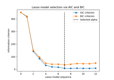
最后,我们可以绘制不同alpha值的AIC和BIC。图中垂直线对应于每个准则选择的alpha。所选alpha对应于AIC或BIC准则的最小值。
ax = results.plot()
ax.vlines(
    alpha_aic,
    results["AIC criterion"].min(),
    results["AIC criterion"].max(),
    label="alpha: AIC estimate",
    linestyles="--",
    color="tab:blue",
)
ax.vlines(
    alpha_bic,
    results["BIC criterion"].min(),
    results["BIC criterion"].max(),
    label="alpha: BIC estimate",
    linestyle="--",
    color="tab:orange",
)
ax.set_xlabel(r"$\alpha$")
ax.set_ylabel("criterion")
ax.set_xscale("log")
ax.legend()
_ = ax.set_title(
    f"Information-criterion for model selection (training time {fit_time:.2f}s)"
)
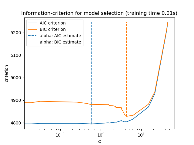
使用信息准则进行模型选择非常快。它依赖于在提供给 fit 的样本内数据集上计算准则。这两个准则都基于训练集误差估计模型的泛化误差,并惩罚这种过于乐观的误差。然而,这种惩罚依赖于对自由度和噪声方差的正确估计。两者都是为大样本(渐近结果)推导的,并且假设模型是正确的,即数据实际上是由该模型生成的。
当问题病态(特征多于样本)时,这些模型也容易失效。此时需要提供噪声方差的估计。
通过交叉验证选择Lasso#
Lasso估计器可以使用不同的求解器实现:坐标下降法和最小角回归。它们在执行速度和数值误差来源方面有所不同。
在scikit-learn中,有两个集成交叉验证的估计器可用:LassoCV 和 LassoLarsCV,它们分别通过坐标下降法和最小角回归解决问题。
在本节的其余部分,我们将介绍这两种方法。对于这两种算法,我们将使用20折交叉验证策略。
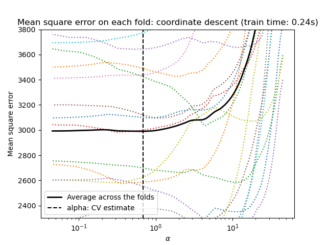
通过坐标下降法的Lasso#
让我们首先使用 LassoCV 进行超参数调优。
from sklearn.linear_model import LassoCV

start_time = time.time()
model = make_pipeline(StandardScaler(), LassoCV(cv=20)).fit(X, y)
fit_time = time.time() - start_time
import matplotlib.pyplot as plt

ymin, ymax = 2300, 3800
lasso = model[-1]
plt.semilogx(lasso.alphas_, lasso.mse_path_, linestyle=":")
plt.plot(
    lasso.alphas_,
    lasso.mse_path_.mean(axis=-1),
    color="black",
    label="Average across the folds",
    linewidth=2,
)
plt.axvline(lasso.alpha_, linestyle="--", color="black", label="alpha: CV estimate")

plt.ylim(ymin, ymax)
plt.xlabel(r"$\alpha$")
plt.ylabel("Mean square error")
plt.legend()
_ = plt.title(
    f"Mean square error on each fold: coordinate descent (train time: {fit_time:.2f}s)"
)
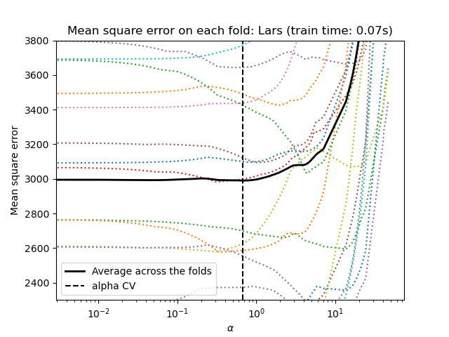
通过最小角回归的Lasso#
让我们首先使用 LassoLarsCV 进行超参数调优。
from sklearn.linear_model import LassoLarsCV

start_time = time.time()
model = make_pipeline(StandardScaler(), LassoLarsCV(cv=20)).fit(X, y)
fit_time = time.time() - start_time
lasso = model[-1]
plt.semilogx(lasso.cv_alphas_, lasso.mse_path_, ":")
plt.semilogx(
    lasso.cv_alphas_,
    lasso.mse_path_.mean(axis=-1),
    color="black",
    label="Average across the folds",
    linewidth=2,
)
plt.axvline(lasso.alpha_, linestyle="--", color="black", label="alpha CV")

plt.ylim(ymin, ymax)
plt.xlabel(r"$\alpha$")
plt.ylabel("Mean square error")
plt.legend()
_ = plt.title(f"Mean square error on each fold: Lars (train time: {fit_time:.2f}s)")
交叉验证方法的总结#
两种算法的结果大致相同。
Lars仅在路径中的每个“扭结”处计算解决方案路径。因此,当“扭结”数量很少时(即特征或样本数量很少时),它非常高效。此外,它能够在不设置任何超参数的情况下计算完整路径。相反,坐标下降法则在预先指定的网格上(此处使用默认设置)计算路径点。因此,如果网格点数量小于路径中的“扭结”数量,则它更高效。如果特征数量非常大且每个交叉验证折叠中都有足够的样本可供选择,这种策略可能会很有趣。在数值误差方面,对于高度相关的变量,Lars会累积更多误差,而坐标下降算法只会在网格上采样路径。
请注意alpha的最佳值在每个折叠中如何变化。这说明了为什么在评估通过交叉验证选择参数的方法的性能时,嵌套交叉验证是一个好的策略:因为仅在未见过测试集上进行最终评估时,这种参数选择可能不是最优的。
结论#
在本教程中,我们介绍了两种选择最佳超参数 alpha 的方法:一种策略仅使用训练集和一些信息准则来找到 alpha 的最优值,另一种策略则基于交叉验证。
在本示例中,两种方法的工作效果相似。样本内超参数选择甚至在计算性能方面也显示出其效率。但是,它只能在样本数量相对于特征数量足够大时使用。
这就是为什么通过交叉验证进行超参数优化是一种安全的策略:它适用于不同的设置。
脚本总运行时间: (0 分钟 0.901 秒)
相关示例