真实数据集上的异常值检测#

此示例说明了在真实数据集上进行鲁棒协方差估计的必要性。这对于异常值检测和更好地理解数据结构都很有用。

我们从 Wine 数据集中选择了两组两个变量，以说明可以使用几种异常值检测工具进行何种分析。为了可视化，我们正在使用二维示例，但应注意，在高维情况下，事情并非如此简单，这一点将会指出。

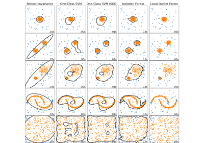
在以下两个示例中，主要结果是非鲁棒的经验协方差估计受到观测值异构结构的强烈影响。尽管鲁棒协方差估计能够关注数据分布的主模式，但它仍然坚持数据应呈高斯分布的假设，导致数据结构估计存在一些偏差，但在一定程度上仍然准确。单类 SVM 不假定数据分布的任何参数形式，因此可以更好地建模数据的复杂形状。

# Authors: The scikit-learn developers
# SPDX-License-Identifier: BSD-3-Clause

第一个示例#

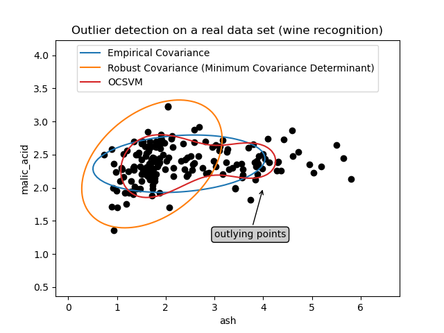
第一个示例说明了当存在异常点时，最小协方差行列式 (Minimum Covariance Determinant) 鲁棒估计器如何帮助集中于相关聚类。此处，经验协方差估计因主聚类外的点而发生偏差。当然，一些筛选工具本可以指出存在两个聚类（支持向量机、高斯混合模型、单变量异常值检测等）。但如果是一个高维示例，这些方法都无法如此轻松地应用。

from sklearn.covariance import EllipticEnvelope
from sklearn.inspection import DecisionBoundaryDisplay
from sklearn.svm import OneClassSVM

estimators = {
    "Empirical Covariance": EllipticEnvelope(support_fraction=1.0, contamination=0.25),
    "Robust Covariance (Minimum Covariance Determinant)": EllipticEnvelope(
        contamination=0.25
    ),
    "OCSVM": OneClassSVM(nu=0.25, gamma=0.35),
}

import matplotlib.lines as mlines
import matplotlib.pyplot as plt

from sklearn.datasets import load_wine

X = load_wine()["data"][:, [1, 2]]  # two clusters

fig, ax = plt.subplots()
colors = ["tab:blue", "tab:orange", "tab:red"]
# Learn a frontier for outlier detection with several classifiers
legend_lines = []
for color, (name, estimator) in zip(colors, estimators.items()):
    estimator.fit(X)
    DecisionBoundaryDisplay.from_estimator(
        estimator,
        X,
        response_method="decision_function",
        plot_method="contour",
        levels=[0],
        colors=color,
        ax=ax,
    )
    legend_lines.append(mlines.Line2D([], [], color=color, label=name))


ax.scatter(X[:, 0], X[:, 1], color="black")
bbox_args = dict(boxstyle="round", fc="0.8")
arrow_args = dict(arrowstyle="->")
ax.annotate(
    "outlying points",
    xy=(4, 2),
    xycoords="data",
    textcoords="data",
    xytext=(3, 1.25),
    bbox=bbox_args,
    arrowprops=arrow_args,
)
ax.legend(handles=legend_lines, loc="upper center")
_ = ax.set(
    xlabel="ash",
    ylabel="malic_acid",
    title="Outlier detection on a real data set (wine recognition)",
)

Outlier detection on a real data set (wine recognition)

第二个示例#

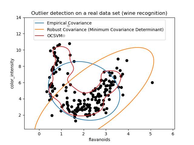
第二个示例展示了最小协方差行列式 (Minimum Covariance Determinant) 鲁棒协方差估计器能够集中于数据分布主模式的能力：尽管由于香蕉形分布协方差难以估计，但位置似乎估计得很好。无论如何，我们可以消除一些异常观测值。单类 SVM 能够捕获真实数据结构，但难点在于调整其核带宽参数，以在数据散布矩阵的形状和数据过拟合风险之间取得良好平衡。

X = load_wine()["data"][:, [6, 9]]  # "banana"-shaped

fig, ax = plt.subplots()
colors = ["tab:blue", "tab:orange", "tab:red"]
# Learn a frontier for outlier detection with several classifiers
legend_lines = []
for color, (name, estimator) in zip(colors, estimators.items()):
    estimator.fit(X)
    DecisionBoundaryDisplay.from_estimator(
        estimator,
        X,
        response_method="decision_function",
        plot_method="contour",
        levels=[0],
        colors=color,
        ax=ax,
    )
    legend_lines.append(mlines.Line2D([], [], color=color, label=name))


ax.scatter(X[:, 0], X[:, 1], color="black")
ax.legend(handles=legend_lines, loc="upper center")
ax.set(
    xlabel="flavanoids",
    ylabel="color_intensity",
    title="Outlier detection on a real data set (wine recognition)",
)

plt.show()

脚本总运行时间： (0 分 0.395 秒)

真实数据集上的异常值检测#

第一个示例#

第二个示例#

本页