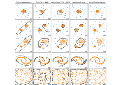
IsolationForest 示例

使用 IsolationForest 进行异常检测的示例。

Isolation Forest 是“孤立树”的集成，它通过递归随机划分来“孤立”观测值，这可以用树结构表示。离群点（outliers）所需划分次数较少，而正常点（inliers）所需划分次数较多。

在本示例中，我们演示了两种可视化在玩具数据集上训练的 Isolation Forest 决策边界的方法。

# Authors: The scikit-learn developers
# SPDX-License-Identifier: BSD-3-Clause

数据生成

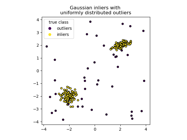
我们通过随机采样 numpy.random.randn 返回的标准正态分布来生成两个聚类（每个聚类包含 n_samples）。其中一个聚类是球形的，另一个略有变形。

为了与 IsolationForest 的表示法保持一致，正常点（即高斯聚类）被赋予真实标签 1，而异常点（使用 numpy.random.uniform 创建）被赋予标签 -1。

import numpy as np

from sklearn.model_selection import train_test_split

n_samples, n_outliers = 120, 40
rng = np.random.RandomState(0)
covariance = np.array([[0.5, -0.1], [0.7, 0.4]])
cluster_1 = 0.4 * rng.randn(n_samples, 2) @ covariance + np.array([2, 2])  # general
cluster_2 = 0.3 * rng.randn(n_samples, 2) + np.array([-2, -2])  # spherical
outliers = rng.uniform(low=-4, high=4, size=(n_outliers, 2))

X = np.concatenate([cluster_1, cluster_2, outliers])
y = np.concatenate(
    [np.ones((2 * n_samples), dtype=int), -np.ones((n_outliers), dtype=int)]
)

X_train, X_test, y_train, y_test = train_test_split(X, y, stratify=y, random_state=42)

我们可以可视化结果聚类

import matplotlib.pyplot as plt

scatter = plt.scatter(X[:, 0], X[:, 1], c=y, s=20, edgecolor="k")
handles, labels = scatter.legend_elements()
plt.axis("square")
plt.legend(handles=handles, labels=["outliers", "inliers"], title="true class")
plt.title("Gaussian inliers with \nuniformly distributed outliers")
plt.show()

模型训练

from sklearn.ensemble import IsolationForest

clf = IsolationForest(max_samples=100, random_state=0)
clf.fit(X_train)

IsolationForest(max_samples=100, random_state=0)

在 Jupyter 环境中，请重新运行此单元格以显示 HTML 表示或信任此笔记本。
在 GitHub 上，HTML 表示无法渲染，请尝试使用 nbviewer.org 加载此页面。

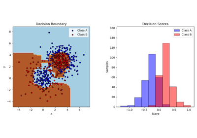
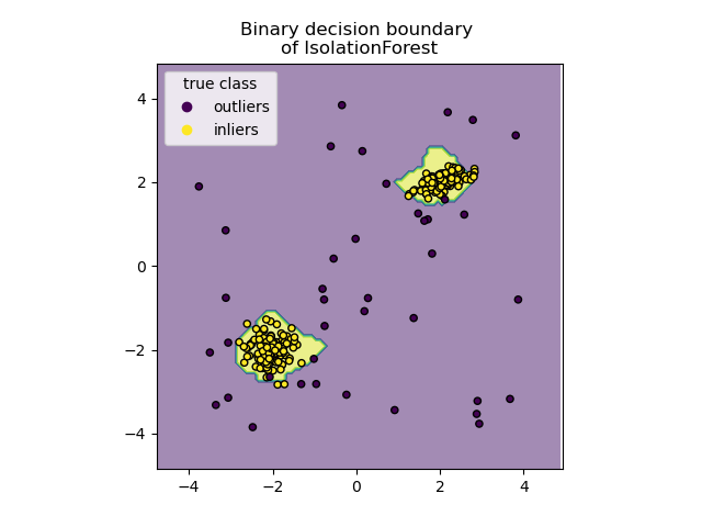
绘制离散决策边界

我们使用 DecisionBoundaryDisplay 类来可视化离散决策边界。背景颜色表示给定区域中的样本是否被预测为异常点。散点图显示真实标签。

import matplotlib.pyplot as plt

from sklearn.inspection import DecisionBoundaryDisplay

disp = DecisionBoundaryDisplay.from_estimator(
    clf,
    X,
    response_method="predict",
    alpha=0.5,
)
disp.ax_.scatter(X[:, 0], X[:, 1], c=y, s=20, edgecolor="k")
disp.ax_.set_title("Binary decision boundary \nof IsolationForest")
plt.axis("square")
plt.legend(handles=handles, labels=["outliers", "inliers"], title="true class")
plt.show()

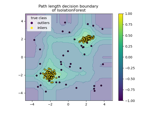
绘制路径长度决策边界

通过设置 response_method="decision_function"，DecisionBoundaryDisplay 的背景表示观测值的正常性度量。该分数由随机树森林中平均路径长度给出，其本身由隔离给定样本所需的叶子深度（或等效地，划分次数）给出。

当随机树森林集体为隔离某些特定样本产生短路径长度时，这些样本极有可能是异常点，并且正常性度量接近 0。类似地，长路径对应于接近 1 的值，并且更可能是正常点。

disp = DecisionBoundaryDisplay.from_estimator(
    clf,
    X,
    response_method="decision_function",
    alpha=0.5,
)
disp.ax_.scatter(X[:, 0], X[:, 1], c=y, s=20, edgecolor="k")
disp.ax_.set_title("Path length decision boundary \nof IsolationForest")
plt.axis("square")
plt.legend(handles=handles, labels=["outliers", "inliers"], title="true class")
plt.colorbar(disp.ax_.collections[1])
plt.show()

相关示例

在玩具数据集上比较用于异常检测的异常检测算法

在玩具数据集上比较用于异常检测的异常检测算法

两类 AdaBoost

两类 AdaBoost

最近邻分类

最近邻分类

Theil-Sen 回归

Theil-Sen 回归