自训练阈值变化的影响#

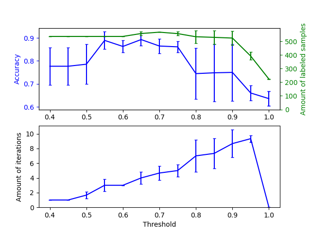
本示例演示了不同阈值对自训练的影响。加载了 breast_cancer 数据集，并删除了标签，使得 569 个样本中只有 50 个样本带有标签。然后使用不同阈值，在该数据集上拟合了一个 SelfTrainingClassifier。

上图显示了分类器在拟合结束时可用的带标签样本数量以及分类器的准确性。下图显示了样本被标记的最后一次迭代。所有值都经过 3 折交叉验证。

在低阈值（[0.4, 0.5] 区间内）下，分类器从置信度低的带标签样本中学习。这些低置信度样本很可能具有不正确的预测标签，因此，基于这些不正确标签进行拟合会导致准确性较差。请注意，分类器几乎标记了所有样本，并且只进行了一次迭代。

对于非常高的阈值（[0.9, 1) 区间内），我们观察到分类器没有增加其数据集（自标记样本的数量为 0）。因此，阈值为 0.9999 时达到的准确性与普通监督分类器所能达到的准确性相同。

最佳准确性介于这两个极端之间，阈值约为 0.7。

# Authors: The scikit-learn developers
# SPDX-License-Identifier: BSD-3-Clause

import matplotlib.pyplot as plt
import numpy as np

from sklearn import datasets
from sklearn.metrics import accuracy_score
from sklearn.model_selection import StratifiedKFold
from sklearn.semi_supervised import SelfTrainingClassifier
from sklearn.svm import SVC
from sklearn.utils import shuffle

n_splits = 3

X, y = datasets.load_breast_cancer(return_X_y=True)
X, y = shuffle(X, y, random_state=42)
y_true = y.copy()
y[50:] = -1
total_samples = y.shape[0]

base_classifier = SVC(probability=True, gamma=0.001, random_state=42)

x_values = np.arange(0.4, 1.05, 0.05)
x_values = np.append(x_values, 0.99999)
scores = np.empty((x_values.shape[0], n_splits))
amount_labeled = np.empty((x_values.shape[0], n_splits))
amount_iterations = np.empty((x_values.shape[0], n_splits))

for i, threshold in enumerate(x_values):
    self_training_clf = SelfTrainingClassifier(base_classifier, threshold=threshold)

    # We need manual cross validation so that we don't treat -1 as a separate
    # class when computing accuracy
    skfolds = StratifiedKFold(n_splits=n_splits)
    for fold, (train_index, test_index) in enumerate(skfolds.split(X, y)):
        X_train = X[train_index]
        y_train = y[train_index]
        X_test = X[test_index]
        y_test = y[test_index]
        y_test_true = y_true[test_index]

        self_training_clf.fit(X_train, y_train)

        # The amount of labeled samples that at the end of fitting
        amount_labeled[i, fold] = (
            total_samples
            - np.unique(self_training_clf.labeled_iter_, return_counts=True)[1][0]
        )
        # The last iteration the classifier labeled a sample in
        amount_iterations[i, fold] = np.max(self_training_clf.labeled_iter_)

        y_pred = self_training_clf.predict(X_test)
        scores[i, fold] = accuracy_score(y_test_true, y_pred)


ax1 = plt.subplot(211)
ax1.errorbar(
    x_values, scores.mean(axis=1), yerr=scores.std(axis=1), capsize=2, color="b"
)
ax1.set_ylabel("Accuracy", color="b")
ax1.tick_params("y", colors="b")

ax2 = ax1.twinx()
ax2.errorbar(
    x_values,
    amount_labeled.mean(axis=1),
    yerr=amount_labeled.std(axis=1),
    capsize=2,
    color="g",
)
ax2.set_ylim(bottom=0)
ax2.set_ylabel("Amount of labeled samples", color="g")
ax2.tick_params("y", colors="g")

ax3 = plt.subplot(212, sharex=ax1)
ax3.errorbar(
    x_values,
    amount_iterations.mean(axis=1),
    yerr=amount_iterations.std(axis=1),
    capsize=2,
    color="b",
)
ax3.set_ylim(bottom=0)
ax3.set_ylabel("Amount of iterations")
ax3.set_xlabel("Threshold")

plt.show()

脚本总运行时间： (0 分钟 4.996 秒)

自训练阈值变化的影响#

本页