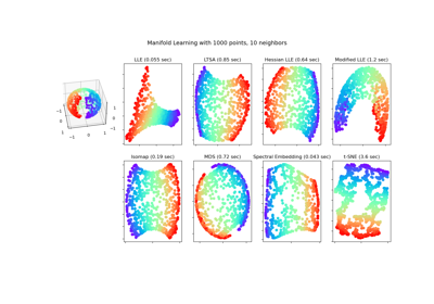
流形学习方法比较#

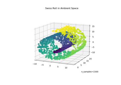
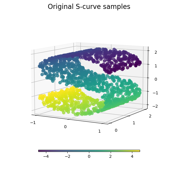
使用各种流形学习方法在S曲线数据集上进行降维的示例。

有关这些算法的讨论和比较，请参见流形模块页面

有关类似示例，其中方法应用于球体数据集，请参见切割球体上的流形学习方法

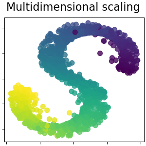
请注意，MDS的目的是找到数据的低维表示（此处为2D），其中距离能够很好地反映原始高维空间中的距离；与其他流形学习算法不同，它不寻求数据在低维空间中的各向同性表示。

# Authors: The scikit-learn developers
# SPDX-License-Identifier: BSD-3-Clause

数据集准备#

我们首先生成S曲线数据集。

import matplotlib.pyplot as plt

# unused but required import for doing 3d projections with matplotlib < 3.2
import mpl_toolkits.mplot3d  # noqa: F401
from matplotlib import ticker

from sklearn import datasets, manifold

n_samples = 1500
S_points, S_color = datasets.make_s_curve(n_samples, random_state=0)

让我们看看原始数据。同时定义一些辅助函数，我们将在后续使用。

def plot_3d(points, points_color, title):
    x, y, z = points.T

    fig, ax = plt.subplots(
        figsize=(6, 6),
        facecolor="white",
        tight_layout=True,
        subplot_kw={"projection": "3d"},
    )
    fig.suptitle(title, size=16)
    col = ax.scatter(x, y, z, c=points_color, s=50, alpha=0.8)
    ax.view_init(azim=-60, elev=9)
    ax.xaxis.set_major_locator(ticker.MultipleLocator(1))
    ax.yaxis.set_major_locator(ticker.MultipleLocator(1))
    ax.zaxis.set_major_locator(ticker.MultipleLocator(1))

    fig.colorbar(col, ax=ax, orientation="horizontal", shrink=0.6, aspect=60, pad=0.01)
    plt.show()


def plot_2d(points, points_color, title):
    fig, ax = plt.subplots(figsize=(3, 3), facecolor="white", constrained_layout=True)
    fig.suptitle(title, size=16)
    add_2d_scatter(ax, points, points_color)
    plt.show()


def add_2d_scatter(ax, points, points_color, title=None):
    x, y = points.T
    ax.scatter(x, y, c=points_color, s=50, alpha=0.8)
    ax.set_title(title)
    ax.xaxis.set_major_formatter(ticker.NullFormatter())
    ax.yaxis.set_major_formatter(ticker.NullFormatter())


plot_3d(S_points, S_color, "Original S-curve samples")

定义流形学习算法#

流形学习是一种非线性降维方法。此任务的算法基于许多数据集的维度只是人为地高这一思想。

在用户指南中阅读更多内容。

n_neighbors = 12  # neighborhood which is used to recover the locally linear structure
n_components = 2  # number of coordinates for the manifold

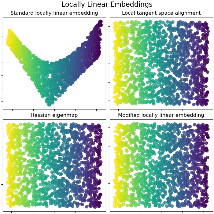
局部线性嵌入#

局部线性嵌入（LLE）可以看作是一系列局部主成分分析，它们进行全局比较以找到最佳非线性嵌入。在用户指南中阅读更多内容。

params = {
    "n_neighbors": n_neighbors,
    "n_components": n_components,
    "eigen_solver": "auto",
    "random_state": 0,
}

lle_standard = manifold.LocallyLinearEmbedding(method="standard", **params)
S_standard = lle_standard.fit_transform(S_points)

lle_ltsa = manifold.LocallyLinearEmbedding(method="ltsa", **params)
S_ltsa = lle_ltsa.fit_transform(S_points)

lle_hessian = manifold.LocallyLinearEmbedding(method="hessian", **params)
S_hessian = lle_hessian.fit_transform(S_points)

lle_mod = manifold.LocallyLinearEmbedding(method="modified", **params)
S_mod = lle_mod.fit_transform(S_points)

fig, axs = plt.subplots(
    nrows=2, ncols=2, figsize=(7, 7), facecolor="white", constrained_layout=True
)
fig.suptitle("Locally Linear Embeddings", size=16)

lle_methods = [
    ("Standard locally linear embedding", S_standard),
    ("Local tangent space alignment", S_ltsa),
    ("Hessian eigenmap", S_hessian),
    ("Modified locally linear embedding", S_mod),
]
for ax, method in zip(axs.flat, lle_methods):
    name, points = method
    add_2d_scatter(ax, points, S_color, name)

plt.show()

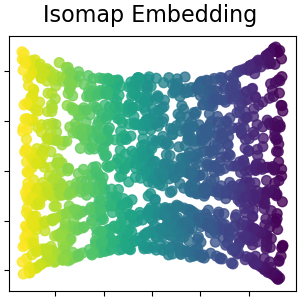
Locally Linear Embeddings, Standard locally linear embedding, Local tangent space alignment, Hessian eigenmap, Modified locally linear embedding

Isomap嵌入#

通过等距映射进行非线性降维。Isomap寻求一种较低维度的嵌入，该嵌入能保持所有点之间的测地线距离。在用户指南中阅读更多内容。

isomap = manifold.Isomap(n_neighbors=n_neighbors, n_components=n_components, p=1)
S_isomap = isomap.fit_transform(S_points)

plot_2d(S_isomap, S_color, "Isomap Embedding")

多维缩放#

多维缩放（MDS）旨在找到数据的低维表示，其中距离能够很好地反映原始高维空间中的距离。在用户指南中阅读更多内容。

md_scaling = manifold.MDS(
    n_components=n_components,
    max_iter=50,
    n_init=1,
    random_state=0,
    normalized_stress=False,
)
S_scaling = md_scaling.fit_transform(S_points)

plot_2d(S_scaling, S_color, "Multidimensional scaling")

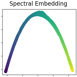
用于非线性降维的谱嵌入#

此实现使用拉普拉斯特征映射，通过图拉普拉斯算子的谱分解找到数据的低维表示。在用户指南中阅读更多内容。

spectral = manifold.SpectralEmbedding(
    n_components=n_components, n_neighbors=n_neighbors, random_state=42
)
S_spectral = spectral.fit_transform(S_points)

plot_2d(S_spectral, S_color, "Spectral Embedding")

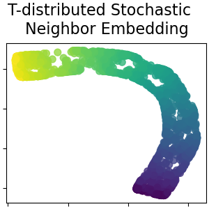
t-分布随机邻域嵌入#

它将数据点之间的相似性转换为联合概率，并试图最小化低维嵌入的联合概率与高维数据之间的Kullback-Leibler散度。t-SNE的代价函数不是凸的，这意味着不同的初始化可能会得到不同的结果。在用户指南中阅读更多内容。

t_sne = manifold.TSNE(
    n_components=n_components,
    perplexity=30,
    init="random",
    max_iter=250,
    random_state=0,
)
S_t_sne = t_sne.fit_transform(S_points)

plot_2d(S_t_sne, S_color, "T-distributed Stochastic  \n Neighbor Embedding")

T-distributed Stochastic Neighbor Embedding

脚本总运行时间： (0 分钟 12.349 秒)