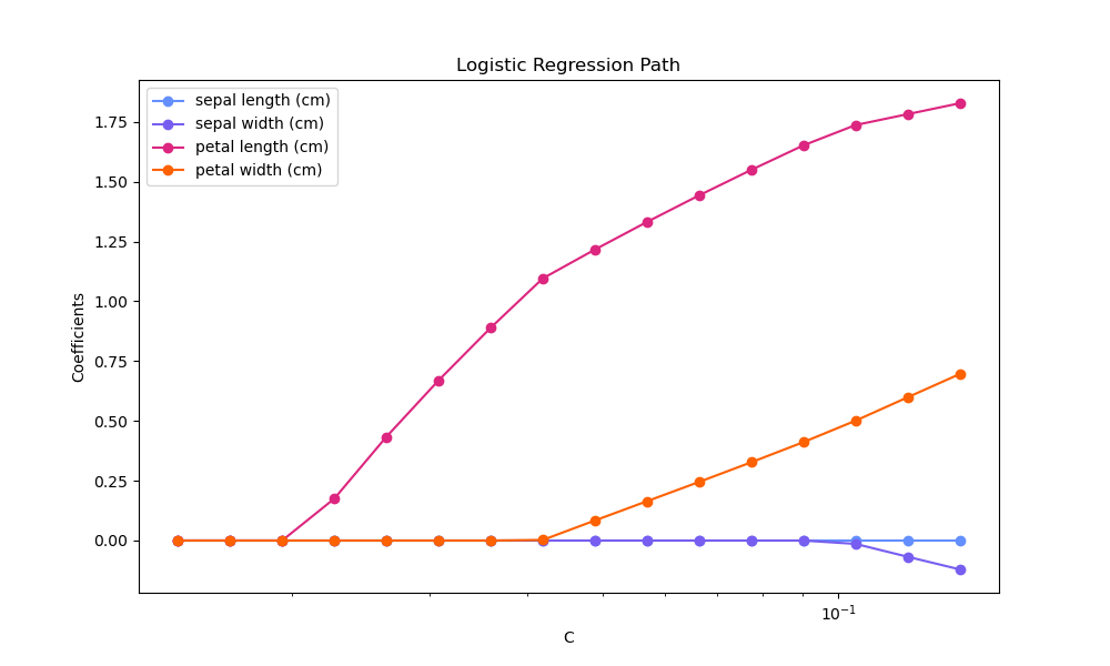
L1正则化逻辑回归的正则化路径#

在源自Iris数据集的二元分类问题上训练L1惩罚逻辑回归模型。

这些模型按照正则化强度从强到弱排序。模型的4个系数被收集并绘制成一个“正则化路径”：在图的左侧（强正则化器），所有系数都精确为0。当正则化逐渐放松时，系数可以依次获得非零值。

这里我们选择liblinear求解器，因为它能够高效地优化带有非平滑、稀疏性L1惩罚的逻辑回归损失。

另请注意，我们将容差值设置得很低，以确保模型在收集系数之前已收敛。

我们还使用了 warm_start=True，这意味着模型的系数被重用以初始化下一次模型拟合，从而加速完整路径的计算。

# Authors: The scikit-learn developers
# SPDX-License-Identifier: BSD-3-Clause

加载数据#

from sklearn import datasets

iris = datasets.load_iris()
X = iris.data
y = iris.target
feature_names = iris.feature_names

这里我们移除第三个类别，使其成为一个二元分类问题

X = X[y != 2]
y = y[y != 2]

计算正则化路径#

import numpy as np

from sklearn.linear_model import LogisticRegression
from sklearn.pipeline import make_pipeline
from sklearn.preprocessing import StandardScaler
from sklearn.svm import l1_min_c

cs = l1_min_c(X, y, loss="log") * np.logspace(0, 1, 16)

创建一个包含 StandardScaler 和 LogisticRegression 的管道，以便在线性模型拟合之前对数据进行归一化，以加速收敛并使系数具有可比性。此外，作为一个副作用，由于数据现在以0为中心，我们无需拟合截距。

clf = make_pipeline(
    StandardScaler(),
    LogisticRegression(
        penalty="l1",
        solver="liblinear",
        tol=1e-6,
        max_iter=int(1e6),
        warm_start=True,
        fit_intercept=False,
    ),
)
coefs_ = []
for c in cs:
    clf.set_params(logisticregression__C=c)
    clf.fit(X, y)
    coefs_.append(clf["logisticregression"].coef_.ravel().copy())

coefs_ = np.array(coefs_)

绘制正则化路径#

import matplotlib.pyplot as plt

# Colorblind-friendly palette (IBM Color Blind Safe palette)
colors = ["#648FFF", "#785EF0", "#DC267F", "#FE6100"]

plt.figure(figsize=(10, 6))
for i in range(coefs_.shape[1]):
    plt.semilogx(cs, coefs_[:, i], marker="o", color=colors[i], label=feature_names[i])

ymin, ymax = plt.ylim()
plt.xlabel("C")
plt.ylabel("Coefficients")
plt.title("Logistic Regression Path")
plt.legend()
plt.axis("tight")
plt.show()

脚本总运行时间： (0 分钟 0.164 秒)

L1正则化逻辑回归的正则化路径#

加载数据#

计算正则化路径#

绘制正则化路径#

此页面