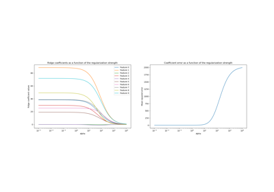
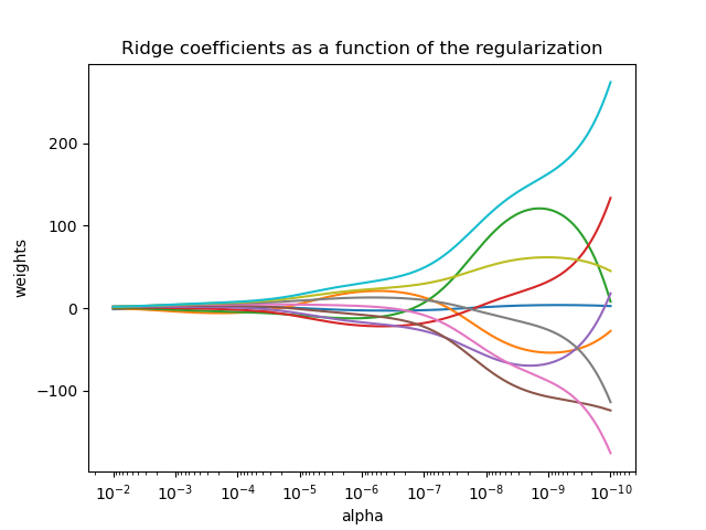
绘制 Ridge 系数作为正则化函数的曲线图#

显示了估计器系数中多重共线性的影响。

Ridge 回归是本示例中使用的估计器。每种颜色代表系数向量的不同特征，并显示为正则化参数的函数。

本示例还展示了将 Ridge 回归应用于严重病态矩阵的实用性。对于此类矩阵，目标变量的微小变化可能导致计算权重产生巨大差异。在这种情况下，设置一定的正则化（alpha）以减少这种变化（噪声）是很有用的。

当 alpha 非常大时，正则化效果会主导平方损失函数，系数趋于零。在路径的末端，当 alpha 趋近于零且解趋近于普通最小二乘时，系数会表现出大的震荡。在实践中，需要对 alpha 进行调整，以使两者之间保持平衡。

# Authors: The scikit-learn developers
# SPDX-License-Identifier: BSD-3-Clause

import matplotlib.pyplot as plt
import numpy as np

from sklearn import linear_model

# X is the 10x10 Hilbert matrix
X = 1.0 / (np.arange(1, 11) + np.arange(0, 10)[:, np.newaxis])
y = np.ones(10)

计算路径#

n_alphas = 200
alphas = np.logspace(-10, -2, n_alphas)

coefs = []
for a in alphas:
    ridge = linear_model.Ridge(alpha=a, fit_intercept=False)
    ridge.fit(X, y)
    coefs.append(ridge.coef_)

显示结果#

ax = plt.gca()

ax.plot(alphas, coefs)
ax.set_xscale("log")
ax.set_xlim(ax.get_xlim()[::-1])  # reverse axis
plt.xlabel("alpha")
plt.ylabel("weights")
plt.title("Ridge coefficients as a function of the regularization")
plt.axis("tight")
plt.show()